Writing your First Distributed Python Application with Ray

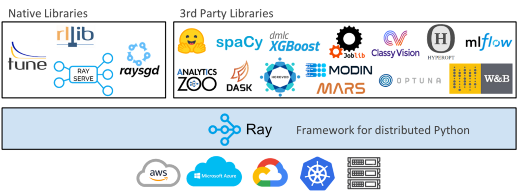
Ray makes parallel and distributed computing work more like you would hope (image source)

Ray is a fast, simple distributed execution framework that makes it easy to scale your applications and to leverage state of the art machine learning libraries. Using Ray, you can take Python code that runs sequentially and transform it into a distributed application with minimal code changes. 

The goal of this tutorial is to explore the following:

• Why should you parallelize and distribute with Ray 

• How to get started with Ray

• Trade-offs in distributed computing (compute cost, memory, I/O, etc)

LinkWhy should you parallelize and distribute with Ray?

As a previous post pointed out, parallel and distributed computing are a staple of modern applications. The problem is that taking existing Python code and trying to parallelize or distribute it can mean rewriting existing code, sometimes from scratch. Additionally modern applications have requirements that existing modules like multiprocessing lack. These requirements include:

• Running the same code on more than one machine

• Building microservices and actors that have state and can communicate

• Graceful handling of machine failures and preemption

• Efficient handling of large objects and numerical data

The Ray library satisfies these requirements and allows you to scale your applications without rewriting them. In order to make parallel & distributed computing simple, Ray takes functions and classes and translates them to the distributed setting as tasks and actors. The rest of this tutorial explores these concepts as well as some important things to consider when building parallel & distributed applications.

While this tutorial explores how Ray makes it easy to parallelize plain Python code, it is important to note that Ray and its ecosystem also make it easy to parallelize python code as well as existing libraries like scikit-learn, XGBoost, LightGBM, PyTorch, and much more.

LinkHow to get started with Ray

LinkTurning Python Functions into Remote Functions (Ray Tasks)

Ray can be installed through pip.

1
pip install 'ray[default]'

Let’s begin our Ray journey by creating a Ray task. This can be done by decorating a normal Python function with @ray.remote. This creates a task which can be scheduled across your laptop's CPU cores (or Ray cluster).

Consider the two functions below which generate Fibonacci sequences (integer sequence characterized by the fact that every number after the first two is the sum of the two preceding ones). The first is a normal python function and the second is a Ray task.

1
2
3
4
5
6
7
8
9
10
11
12
13
14
15
16
17
18
19
20
21
22
23
24
import os
import time
import ray

# Normal Python
def fibonacci_local(sequence_size):
    fibonacci = []
    for i in range(0, sequence_size):
        if i < 2:
            fibonacci.append(i)
            continue
        fibonacci.append(fibonacci[i-1]+fibonacci[i-2])
    return sequence_size

# Ray task
@ray.remote
def fibonacci_distributed(sequence_size):
    fibonacci = []
    for i in range(0, sequence_size):
        if i < 2:
            fibonacci.append(i)
            continue
        fibonacci.append(fibonacci[i-1]+fibonacci[i-2])
    return sequence_size

There are a couple of things to note regarding these two functions. First, they are identical except for the @ray.remote decorator on the fibonacci_distributed function.

The second thing to note is the small return value. They are not returning the Fibonacci sequences themselves, but the sequence size, which is an integer.  This is important, because it might lessen the value of a distributed function by designing it so that it requires or returns a lot of data (parameters). Engineers often refer to this as the input/output (IO) of a distributed function.

LinkComparing Local vs Remote Performance

The functions in this section will allow us to compare how long it takes to generate multiple long Fibonacci sequences both locally and in parallel. It is important to note that both functions below utilize os.cpu_count() which returns the number of CPUs in the system.

1
os.cpu_count()

The machine used in this tutorial has eight CPUs which means that each function below will generate 8 Fibonacci sequences.

1
2
3
4
5
6
7
8
9
10
11
12
13
14
15
16

# Normal Python
def run_local(sequence_size):
    start_time = time.time()
    results = [fibonacci_local(sequence_size) for _ in range(os.cpu_count())]
    duration = time.time() - start_time
    print('Sequence size: {}, Local execution time: {}'.format(sequence_size, duration))

# Ray
def run_remote(sequence_size):
    # Starting Ray
    ray.init()
    start_time = time.time()
    results = ray.get([fibonacci_distributed.remote(sequence_size) for _ in range(os.cpu_count())])
    duration = time.time() - start_time
    print('Sequence size: {}, Remote execution time: {}'.format(sequence_size, duration))  

Before getting into how the code for run_local and run_remote work, let's run both of these functions to see how long it takes to generate multiple 100000 number Fibonacci sequences both locally and remotely.

1
2
run_local(100000)
run_remote(100000)

The run_remote function parallelized the computation across multiple cpus which resulted in a smaller processing time (1.76s vs 4.20s).

LinkThe Ray API 

In order to better understand why run_remote was faster, let's briefly go over the code and along the way explain how the Ray API works.

The ray.init() command starts all of the relevant Ray processes. By default, Ray creates one worker process per CPU core. If you would want to run Ray on a cluster, you would need to pass in a cluster address with something like ray.init(address= 'InsertAddressHere').

fibonacci_distributed.remote(100000)

Calling fibonacci_distributed.remote(sequence_size) immediately returns a future and not the return value of the function. The actual function execution will take place in the background. Since it returns immediately, each function call can be executed in parallel. This makes generating those multiple 100000 long fibonacci sequences take less time.

ray.get retrieves the resulting value from the task when it completes.

Finally, it is important to note that when the process calling ray.init() terminates, the Ray runtime will also terminate. Note that if you try and run ray.init() more than once you may get a RuntimeError (Maybe you called ray.init twice by accident?). This can be solved by using ray.shutdown()

1
2
# To explicitly stop or restart Ray, use the shutdown API
ray.shutdown()

LinkRay Dashboard

Ray comes with a dashboard that is available at http://127.0.0.1:8265 after you call the ray.init function. 

Among other things, the dashboard lets you:

• Understand Ray memory utilization and debug memory errors.

• See per-actor resource usage, executed tasks, logs, and more.

• View cluster metrics.

• Kill actors and profile your Ray jobs.

• See errors and exceptions at a glance.

• View logs across many machines in a single pane.

• See Ray Tune jobs and trial information.

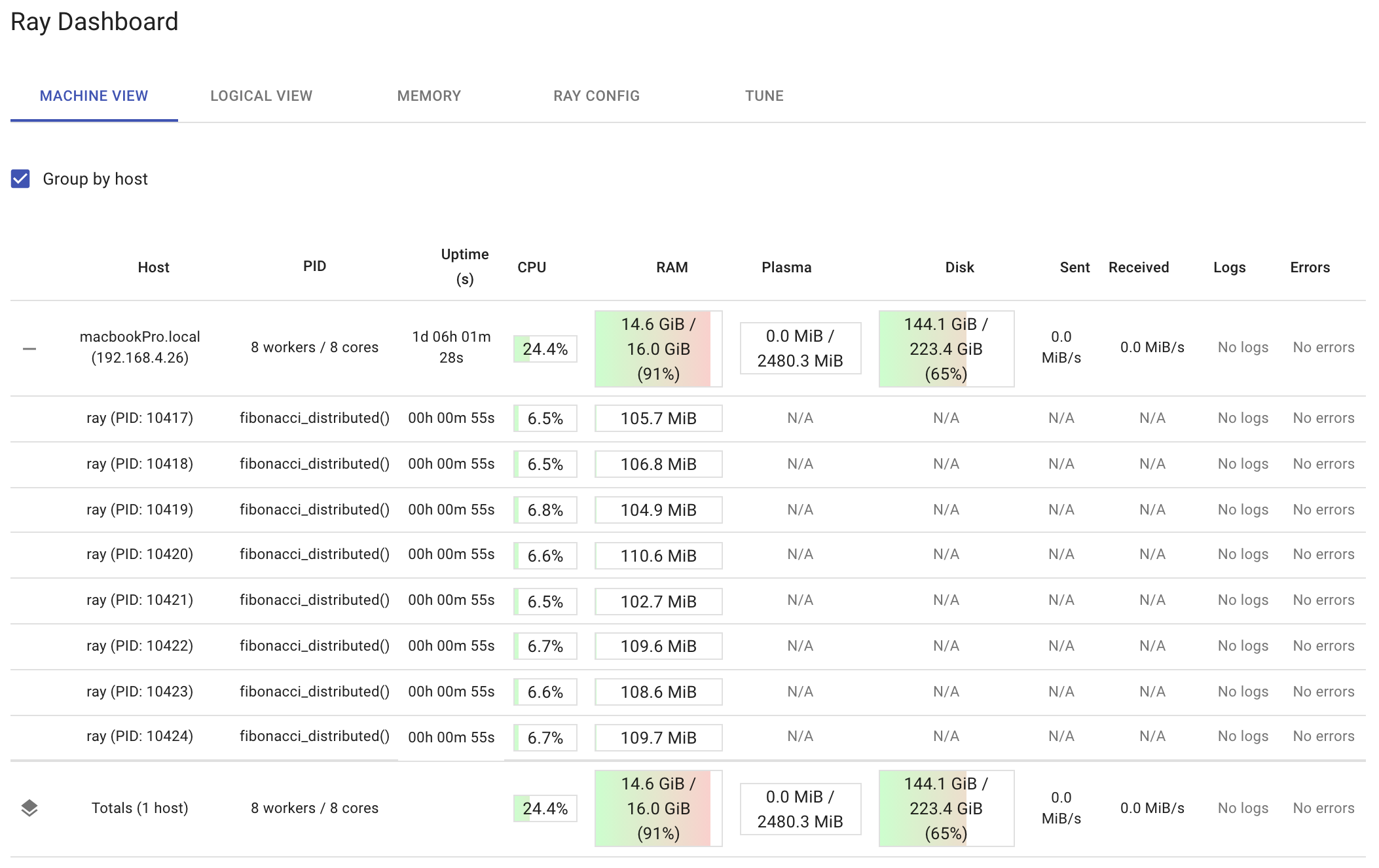
The dashboard below shows the resource utilization on a per-node and per-worker basis after running run_remote(200000). Notice how the dashboard shows the function fibonacci_distributed that’s running in each worker. It’s a good idea to observe your distributed functions while they are running. That way, if you see one worker doing all the work, then you may be using the ray.get function incorrectly. Also, if you see your total CPU utilization getting close to 100 percent, you may be doing too much.

LinkTrade-offs in distributed computing

This tutorial used Fibonacci sequences because they provide several options for tweaking computing and IO. You can alter the amount of computing that each function call requires by increasing and decreasing the sequence size. The greater the sequence size, the more computing you need to generate the sequence, whereas the smaller the sequence size, the less computing you need. If the computation you distribute is too small, the overhead of Ray would dominate the total processing time, and you wouldn’t get any value out of distributing our functions.

IO is also essential when distributing functions. If you modified these functions to return the sequences they calculate, the IO would increase as the sequence size increased. At some point, the time needed to transmit the data would dominate the total time required to complete the multiple calls to the distributed function. This is important if you are distributing your functions over a cluster. This would require the use of a network, and network calls are more costly than the interprocess communication used in this tutorial.

Therefore, it is recommended that you try to experiment with both the distributed Fibonacci function and the local Fibonacci function. Try to determine the minimum sequence size needed to benefit from a remote function. Once you figure out the computing, play with the IO to see what happens to overall performance. Distributed architectures, regardless of the tool you use, work best when they don’t have to move a lot of data around.

Fortunately, a major benefit of Ray is the ability to maintain entire objects remotely. This helps mitigate the IO problem. Let’s look at that next.

LinkRemote Objects as Actors

Just as Ray translates Python functions to the distributed setting as tasks, Ray translates Python classes to the distributed setting as actors. Ray provides actors to allow you to parallelize an instance of a class. Code wise, all you need to add to a Python class is the @ray.remote decorator to make it an actor. When you make an instance of that class, Ray creates a new actor which is a process that runs in the cluster and holds a copy of the object.

Since they are remote objects, they can hold data, and their methods can manipulate that data. This helps cut down on interprocess communication. Consider using an actor if you find yourself writing too many tasks that return data, which in turn are sent to other tasks.

Let’s now look at the actor below.

1
2
3
4
5
6
7
8
9
10
11
12
13
14
15
16
17
18
19
20
21
22
23
24
25
26
27
28
29
30
31
32
33
34
35
36
37
38
39
40
41
42
43
44
45
46
47
48
49
50
51
52
53
54
55
56
57
58
from collections import namedtuple
import csv
import tarfile
import time

import ray

@ray.remote
class GSODActor():

    def __init__(self, year, high_temp):
        self.high_temp = float(high_temp)
        self.high_temp_count = None
        self.rows = []
        self.stations = None
        self.year = year

    def get_row_count(self):
        return len(self.rows)

    def get_high_temp_count(self):
        if self.high_temp_count is None:
            filtered = [l for l in self.rows if float(l.TEMP) >= self.high_temp]
            self.high_temp_count = len(filtered)
        return self.high_temp_count

    def get_station_count(self):
        return len(self.stations)

    def get_stations(self):
        return self.stations

    def get_high_temp_count(self, stations):
        filtered_rows = [l for l in self.rows if float(l.TEMP) >= self.high_temp and l.STATION in stations]
        return len(filtered_rows)

    def load_data(self):
        file_name = self.year + '.tar.gz'
        row = namedtuple('Row', ('STATION', 'DATE', 'LATITUDE', 'LONGITUDE', 'ELEVATION', 'NAME', 'TEMP', 'TEMP_ATTRIBUTES', 'DEWP',
                                 'DEWP_ATTRIBUTES', 'SLP', 'SLP_ATTRIBUTES', 'STP', 'STP_ATTRIBUTES', 'VISIB', 'VISIB_ATTRIBUTES',
                                 'WDSP', 'WDSP_ATTRIBUTES', 'MXSPD', 
                                 'GUST', 'MAX', 'MAX_ATTRIBUTES', 'MIN', 'MIN_ATTRIBUTES', 'PRCP',
                                 'PRCP_ATTRIBUTES', 'SNDP', 'FRSHTT'))

        tar = tarfile.open(file_name, 'r:gz')
        for member in tar.getmembers():
            member_handle = tar.extractfile(member)
            byte_data = member_handle.read()
            decoded_string = byte_data.decode()
            lines = decoded_string.splitlines()
            reader = csv.reader(lines, delimiter=',')

            # Get all the rows in the member. Skip the header.
            _ = next(reader)
            file_rows = [row(*l) for l in reader]
            self.rows += file_rows

        self.stations = {l.STATION for l in self.rows}

The code above can be used to load and manipulate data from a public dataset known as the Global Surface Summary of the Day (GSOD). The dataset is managed by the National Oceanic and Atmospheric Administration (NOAA) and it is freely available on their site. NOAA currently maintains data from over 9,000 stations worldwide and the GSOD dataset contains daily summary information from these stations. There is one gzip file for each year from 1929 to 2020. For this tutorial, you only need to download the files for 1980 and 2020. 

The goal of this actor experiment is to compute how many readings from 1980 and 2020 were 100 degrees or greater and determine if 2020 had more extreme temperatures than 1980. In order to implement a fair comparison, only stations that existed in both 1980 and 2020 should be considered. So, the logic of this experiment looks like this:

• Load 1980 data.

• Load 2020 data.

• Get a list of stations that existed in 1980.

• Get a list of stations that existed in 2020.

• Determine the intersection of stations.

• Get the number of readings that were 100 degrees or greater from the intersection of stations during 1980.

• Get the number of readings that were 100 degrees or greater from the intersection of stations during 2020.

• Print the results.

The problem is that this logic is completely sequential; one thing only happens after another. With Ray, a lot of this logic can be done in parallel.

The table below shows a more parallelizable logic.

Writing out the logic in this fashion is an excellent way of making sure you are executing everything that you can in a parallelizable way. The code below implements this logic.

1
2
3
4
5
6
7
8
9
10
11
12
13
14
15
16
17
18
19
20
21
22
23
24
25
26
27
# Code assumes you have the 1980.tar.gz and 2020.tar.gz files in your current working directory.
def compare_years(year1, year2, high_temp):

    # if you know that you need fewer than the default number of workers,
    # you can modify the num_cpus parameter
    ray.init(num_cpus=2)

    # Create actor processes
    gsod_y1 = GSODActor.remote(year1, high_temp)
    gsod_y2 = GSODActor.remote(year2, high_temp)

    ray.get([gsod_y1.load_data.remote(), gsod_y2.load_data.remote()])

    y1_stations, y2_stations = ray.get([gsod_y1.get_stations.remote(),
               	                    gsod_y2.get_stations.remote()])

    intersection = set.intersection(y1_stations, y2_stations)

    y1_count, y2_count = ray.get([gsod_y1.get_high_temp_count.remote(intersection),
                                  gsod_y2.get_high_temp_count.remote(intersection)])

    print('Number of stations in common: {}'.format(len(intersection)))
    print('{} - High temp count for common stations: {}'.format(year1, y1_count))
    print('{} - High temp count for common stations: {}'.format(year2, y2_count))

#Running the code below will output which year had more extreme temperatures
compare_years('1980', '2020', 100)

There are a couple important things to mention about the code above. First, putting the @ray.remote decorator at the class level enabled all class methods to be called remotely. Second, the code above utilizes two actor processes (gsod_y1 and gsod_y2) which can execute methods in parallel (though each actor can only execute one method at a time). This is what enabled the loading and processing of the 1980 and 2020 data at the same time.

LinkConclusion

Ray is a fast, simple distributed execution framework that makes it easy to scale your applications and to leverage state of the art machine learning libraries.  This tutorial showed how using Ray makes it easy to take your existing Python code that runs sequentially and transform it into a distributed application with minimal code changes. While the experiments here were all performed on the same machine, Ray also makes it easy to scale your Python code on every major cloud provider. If you’re interested in learning more about Ray, check out the Ray project on GitHub, follow @raydistributed on twitter, and sign up for the Ray newsletter.