What is hyperparameter tuning?

💡 This blog post is part 1 in our series on hyperparameter tuning. If you're looking for a hands-on look at different tuning methods, be sure to check out part 2, How to tune hyperparameters on XGBoost, and part 3, How to distribute hyperparameter tuning using Ray Tune.

Hyperparameter tuning is an essential part of controlling the behavior of a machine learning model. If we don’t correctly tune our hyperparameters, our estimated model parameters produce suboptimal results, as they don’t minimize the loss function. This means our model makes more errors. In practice, key indicators like the accuracy or the confusion matrix will be worse.

In this article, we’ll explore some examples of hyperparameters and delve into a few models for tuning hyperparameters. Then, in the following two articles of this series, we’ll demonstrate how to tune hyperparameters on XGBoost and how to perform distributed hyperparameter tuning.

LinkWhat are hyperparameters?

In machine learning, we need to differentiate between parameters and hyperparameters. A learning algorithm learns or estimates model parameters for the given data set, then continues updating these values as it continues to learn. After learning is complete, these parameters become part of the model. For example, each weight and bias in a neural network is a parameter.

Hyperparameters, on the other hand, are specific to the algorithm itself, so we can’t calculate their values from the data. We use hyperparameters to calculate the model parameters. Different hyperparameter values produce different model parameter values for a given data set.

Hyperparameter tuning consists of finding a set of optimal hyperparameter values for a learning algorithm while applying this optimized algorithm to any data set. That combination of hyperparameters maximizes the model’s performance, minimizing a predefined loss function to produce better results with fewer errors. Note that the learning algorithm optimizes the loss based on the input data and tries to find an optimal solution within the given setting. However, hyperparameters describe this setting exactly.

For instance, if we work on natural language processing (NLP) models, we probably use neural networks, support-vector machines (SVMs), Bayesian networks, and Extreme Gradient Boosting (XGB) for tuning parameters.

We’ll discuss how to perform hyperparameter tuning in detail later.

LinkHyperparameter types

Some important hyperparameters that require tuning in neural networks are:

• Number of hidden layers: It’s a trade-off between keeping our neural network as simple as possible (fast and generalized) and classifying our input data correctly. We can start with values of four to six and check our data’s prediction accuracy when we increase or decrease this hyperparameter.

• Number of nodes/neurons per layer: More isn't always better when determining how many neurons to use per layer. Increasing neuron count can help, up to a point. But layers that are too wide may memorize the training dataset, causing the network to be less accurate on new data.

• Learning rate: Model parameters are adjusted iteratively — and the learning rate controls the size of the adjustment at each step. The lower the learning rate, the lower the changes to parameter estimates are. This means that it takes a longer time (and more data) to fit the model — but it also means that it is more likely that we actually find the minimum loss.

• Momentum: Momentum helps us avoid falling into local minima by resisting rapid changes to parameter values. It encourages parameters to keep changing in the direction they were already changing, which helps prevent zig-zagging on every iteration. Aim to start with low momentum values and adjust upward as needed.

We consider these essential hyperparameters for tuning SVMs:

• C: A trade-off between a smooth decision boundary (more generic) and a neat decision boundary (more accurate for the training data). A low value may cause the model to incorrectly classify some training data, while a high value may cause the model to incur overfitting. Overfitting creates an analysis too specific for the current data set and possibly unfit for future data and unreliable for future observations.

• Gamma: The inverse of the influence radius of data samples we selected as support vectors. High values indicate the small radius of influence and small decision boundaries that do not consider relatively close data samples. These high values cause overfitting. Low values indicate the significant effect of distant data samples, so the model can’t capture the correct decision boundaries from the data set.

Important hyperparameters that need tuning for XGBoost are:

• max_depth and min_child_weight: This controls the tree architecture. max_depth defines the maximum number of nodes from the root to the farthest leaf (the default number is 6). min_child_weight is the minimum weight required to create a new node in the tree.

• learning_rate: This determines the amount of correction at each step, given that each boosting round corrects the previous round’s errors. learning_rate takes values from 0 to 1, and the default value is 0.3.

• n_estimators: This defines the number of trees in the ensemble. The default value is 100. Note that if we were using vanilla XGBoost instead of scikit-learn, we'd use num_boost_rounds instead of n_estimators.

• colsample_bytree and subsample: This controls the data set samples that each round uses. These hyperparameters are helpful to avoid overfitting. subsample is the fraction of samples used, with a value from 0 to 1 and a default value of 1. colsample_bytree defines the fraction of columns (features) and takes numbers from 0 to 1, with a default value of 1.

In these examples, hyperparameters tending toward one extreme or the other can negatively affect our model’s ability to make predictions. The trick is to find just the right value for each hyperparameter, so our model performs well and produces the best possible results.

LinkMethods for tuning hyperparameters

Now that we understand what hyperparameters are and the importance of tuning them, we need to know how to choose their optimal values. We can find these optimal hyperparameter values using manual or automated methods.

When tuning hyperparameters manually, we typically start using the default recommended values or rules of thumb, then search through a range of values using trial-and-error. But manual tuning is a tedious and time-consuming approach. It isn’t practical when there are many hyperparameters with a wide range.

Automated hyperparameter tuning methods use an algorithm to search for the optimal values. Some of today’s most popular automated methods are grid search, random search, and Bayesian optimization. Let’s explore these methods in detail.

LinkGrid search

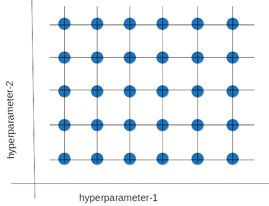
Grid search is a sort of “brute force” hyperparameter tuning method. We create a grid of possible discrete hyperparameter values then fit the model with every possible combination. We record the model performance for each set then select the combination that has produced the best performance.

Grid search is a hyperparameter tuning method in which we create a grid of possible discrete hyperparameter values, then fit the model with every possible combination.

Grid search is an exhaustive algorithm that can find the best combination of hyperparameters. However, the drawback is that it’s slow. Fitting the model with every possible combination usually requires a high computation capacity and significant time, which may not be available.

LinkRandom search

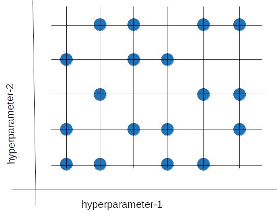
The random search method (as its name implies) chooses values randomly rather than using a predefined set of values like the grid search method. 

Random search tries a random combination of hyperparameters in each iteration and records the model performance. After several iterations, it returns the mix that produced the best result.

Random search tries a random combination of hyperparameters in each iteration and records the model performance. After several iterations, it returns the mix that produced the best result.

Random search is appropriate when we have several hyperparameters with relatively large search domains. We can make discrete ranges (for instance, [5-100] in steps of 5) and still get a reasonably good set of combinations.

The benefit is that random search typically requires less time than grid search to return a comparable result. It also ensures we don't end up with a model that's biased toward value sets arbitrarily chosen by users. Its drawback is that the result may not be the best possible hyperparameter combination.

LinkBayesian optimization

Grid search and random search are relatively inefficient because they often evaluate many unsuitable hyperparameter combinations. They don’t take into account the previous iterations’ results when choosing the next hyperparameters.

The Bayesian optimization method takes a different approach. This method treats the search for the optimal hyperparameters as an optimization problem. When choosing the next hyperparameter combination, this method considers the previous evaluation results. It then applies a probabilistic function to select the combination that will probably yield the best results. This method discovers a fairly good hyperparameter combination in relatively few iterations. 

Data scientists choose a probabilistic model when the objective function is unknown. That is, there is no analytical expression to maximize or minimize. The data scientists apply the learning algorithm to a data set, use the algorithm’s results to define the objective function, and take the various hyperparameter combinations as the input domain.

The probabilistic model is based on past evaluation results. It estimates the probability of a hyperparameter combination’s objective function result:

P( result | hyperparameters )

This probabilistic model is a “surrogate” of the objective function. The objective function can be, for instance, the root-mean-square error (RMSE). We calculate the objective function using the training data with the hyperparameter combination. We try to optimize it (maximize or minimize, depending on the objective function selected).

Applying the probabilistic model to the hyperparameters is computationally inexpensive compared to the objective function, so this method typically updates and improves the surrogate probability model every time the objective function runs. Better hyperparameter predictions decrease the number of objective function evaluations we need to achieve a good result.

Gaussian processes, random forest regression, and tree-structured Parzen estimators (TPE) are surrogate model examples.

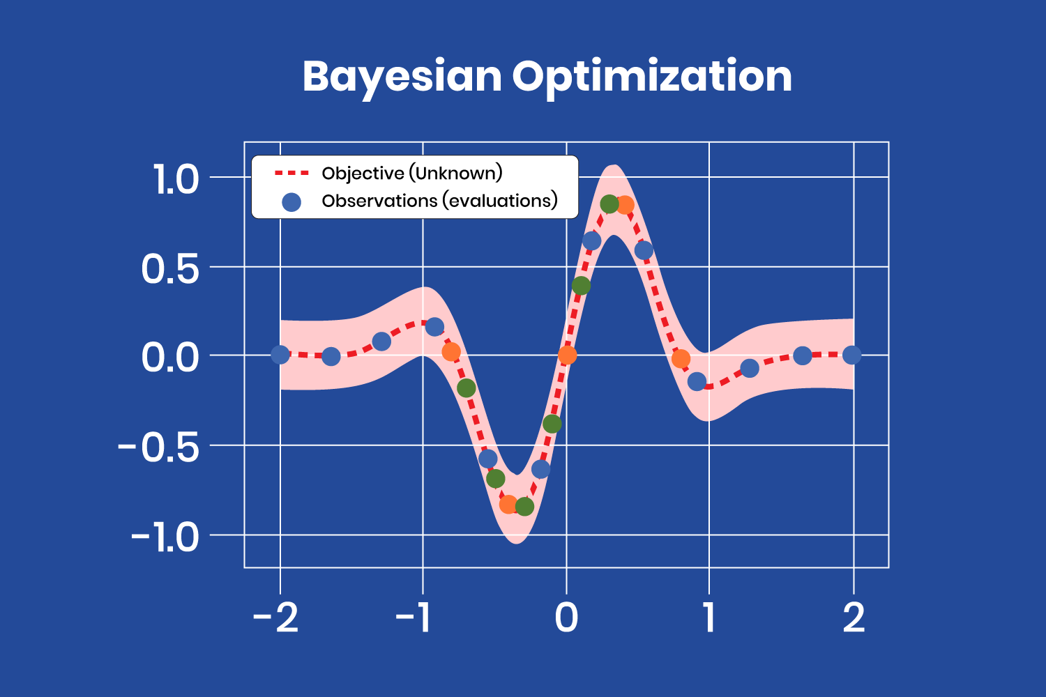
The figure below shows how a surrogate function finds the minimum of the “objective” function, where the “objective” function is unknown.

The Bayesian optimization method treats the search for the optimal hyperparameters as an optimization problem.

After a few iterations, with the evaluations (observations) obtained from the “objective” function, the surrogate model finds the minimum at the coordinates x=-0.35 and y=-0.8. Note that there are several evaluations close to that point, corresponding to the latest iterations, as the model has almost found the minimum and produces similar values (different color points correspond to different iterations).

The Bayesian optimization model is complex to implement. Fortunately, we can use off-the-shelf libraries like Ray Tune to simplify the process. It’s worthwhile to use this type of model because it finds an adequate hyperparameter combination in relatively few iterations.

Bayesian optimization is helpful when the objective function is costly in computing resources and time. A drawback compared to grid search or random search is that we must compute Bayesian optimization sequentially (where the next iteration depends on the previous one), so it doesn’t allow distributed processing. So, Bayesian optimization takes longer yet uses fewer computational resources.

LinkNext steps

We should perform model hyperparameter tuning to ensure good results from our machine learning model and data. We can choose from three hyperparameter tuning methods — grid search, random search, and Bayesian optimization. If evaluating our model with training data will be quick, we can choose the grid search method. Otherwise, we should select random search or Bayesian optimization to save time and computing resources.

In the next article in this series, we’ll demonstrate hands-on how to tune hyperparameters on XGBoost. We’ll build and optimize a machine learning model to identify images of digits.