In a previous blog, we showed how Ray Data can provide speedups over SageMaker and frameworks like Apache Spark for large-scale batch inference workloads. This blog post delves further into how Ray Data streaming works and how to use it for your own ML pipelines.

Some of the most demanding machine learning (ML) use cases we have encountered involve pipelines that span both CPU and GPU devices in distributed environments. These situations arise in various workloads, including:

• Batch inference, which involves a CPU-intensive preprocessing stage (e.g., video decoding or image resizing) before utilizing a GPU-intensive model to make predictions.

• Distributed training, where similar CPU-heavy transformations are required to prepare or augment the dataset prior to GPU training.

Interestingly, in many of these workloads, the preprocessing steps often prove to be the bottleneck. This can happen when preprocessing requires parallelism across multiple nodes and significant memory to buffer results between the CPU and GPU.

For instance, consider the decoding of compressed images in memory. A typical JPEG decompression ratio is 10:1, which implies that the output memory size may be ten times that of the input, resulting in substantial memory pressure in addition to CPU load. The challenges become more complex with other data modalities, such as video; for example, H264 can decompress at a 2000:1 ratio, producing 200GB of frame outputs for a 100MB file input. This means that practitioners trying to offload CPU-heavy preprocessing onto multiple CPUs or machines have to deal with intermediate results that are far larger than their already sizable source datasets:

Figure 1. Decoding of compressed images with large images spilled to disk

Executed naively, these compute and memory-intensive workloads fail to fully utilize expensive GPU hardware. For example, we could buffer 200GB of frame outputs on disk, but that could add minutes of overheads. Even if this is overlapped with GPU computation, we can end up with long pauses on the GPU. This motivates fully streamed execution in the cluster setting, which avoids such delays by streaming intermediate data through cluster memory:

Figure 2. Decoding intermediate data streamed through memory

In this blog post, we guide you through our development of a versatile streaming backend for Ray Data, and show examples of how to implement the demanding use cases mentioned earlier. We discuss the performance benefits of implementing pipelined execution across CPUs and GPUs compared to bulk processing, and discuss its broader applicability to various workloads, including distributed training.

LinkPipelined execution in a cluster

To understand the necessity and advantages of pipelined (or streaming) execution across CPU and GPU devices, let's first examine how a bulk synchronous parallel (BSP) framework might handle batch inference. Because of its simplicity and generality, BSP is a common way frameworks (e.g., MapReduce, Apache Spark) parallelize distributed computations.

Note that pipelining within a single machine is already commonly used in data loading libraries such as Torch DataLoader or Petastorm. Here, we discuss pipelining computations across an entire cluster of machines.

A typical batch inference job consists of the following operations:

Figure 3. A typical batch inference job sequential operations

To implement such an inference job, you'd write the code using Ray Data (or another similar framework):

1import ray
2
3# Define model and preprocessor.
4model = ...
5preprocess_fn = ...
6
7# Define the inference function.
8def model_fn(batch: Dict[str, np.ndarray]):
9    return {"results": model(batch)}
10
11# The following snippet implements the pipeline.
12ray.data.read_parquet(...) \           # 1. Load
13    .map_batches(preprocess_fn) \      # 2. Preprocess
14    .map_batches(model_fn) \           # 3. Inference
15    .write_parquet(...)                # 4. Save
16

In a BSP framework, each of these operations can be modeled as a 1:1 transformation, which can be fused together into a single stage. Each task within the stage will execute the mentioned operations locally in sequence:

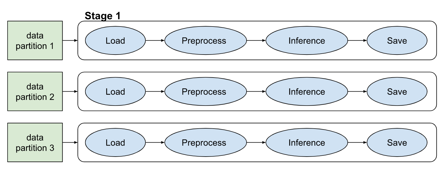Figure 4. BSP framework operations modeled as a 1:1 transformation

This execution strategy is memory optimal, as there is no intermediate data and execution is inherently pipelined (since there is only a single stage). However, challenges emerge in a heterogeneous setting, where certain pipeline steps may prefer to run on CPUs or GPUs independently. In Ray Data, such inference pipelines are expressed with transformations that launch actors scheduled onto GPUs (num_gpus=1 and compute=ActorPoolStrategy):

1import ray
2from ray.data import ActorPoolStrategy
3
4Model = ...
5preprocess_fn = ...
6
7# Define the model as a stateful class with cached setup.
8class MyModelCallableCls:
9    def __init__(self):
10        self.model = Model(...)
11
12    def __call__(self, batch: Dict[str, np.ndarray]) ->
13        return {"results": self.model(batch)}
14
15# Modify the pipeline to use GPU actors.
16ray.data.read_parquet(...) \
17    .map_batches(preprocess_fn) \
18    .map_batches(
19          MyModelCallableCls,
20          num_gpus=1,
21          compute=ActorPoolStrategy(size=N)) \
22    .write_parquet(...)

In the above code snippet, the load and preprocessing steps run on CPU (Stage 1), inference runs on GPUs (Stage 2), and then the result saving runs on CPU again (Stage 3). This configuration leads to spilling of data to remote storage when intermediate results (e.g., decoded video frames) exceed cluster memory sizes. Hence, we see that BSP is not memory optimal for heterogeneous workloads:

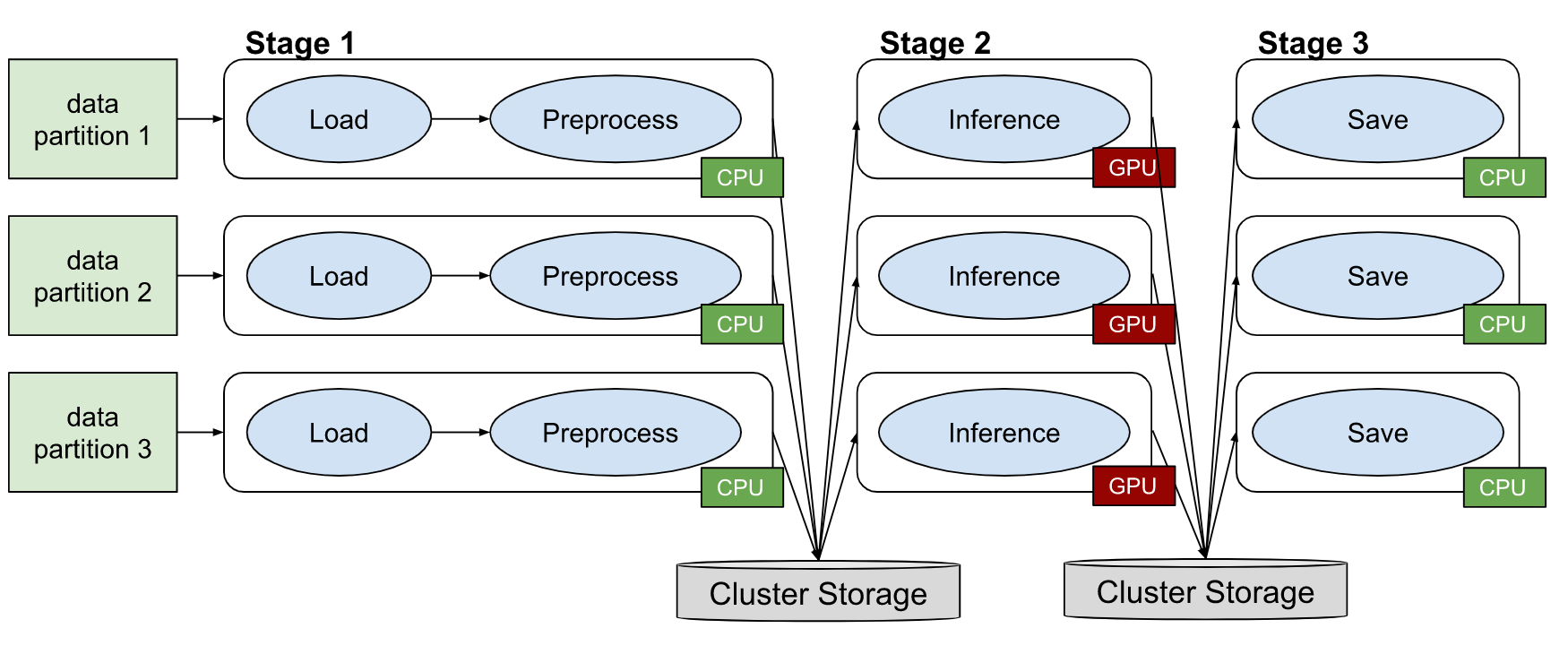Figure 5. BSP is not memory optimal for heterogeneous workloads

These unnecessary overheads can be avoided with end-to-end pipelining (i.e., streaming) across the cluster, which we present in the next section.

LinkRay Data streaming

In Ray 2.4, we've changed the default execution strategy of Ray Data to streaming from bulk synchronous. These streaming Datasets are fully backwards compatible with the existing API, i.e., they can be transformed lazily with map operations, support shuffle operations, and also caching / materialization in memory:

1# Create a dataset over parquet files
2ds: ray.data.Dataset = ray.data.read_parquet(...)
3
4# Transform the dataset
5ds = ds.map_batches(my_preprocess_fn)
6ds = ds.map_batches(my_model_fn)
7
8# Iterate over dataset batches in streaming fashion
9for batch in ds.iter_batches():
10   print(batch)
11
12# Materialize all contents of the dataset in memory
13ds = ds.materialize()

In other words, the Ray Data API now leverages streaming execution for improved performance on large datasets, with the same simple transformation API as in previous Ray versions.

LinkVideo processing example

To more fully understand the capabilities of this API, let's walk through what this looks like in an example video processing pipeline. In the pipeline, we'll first decode video frames, annotate each frame with an ML model, apply a classification model to the annotated frames, and then save the results to JSON:

Figure 6. A pipeline decoding video frames, annotating frames, applying classification, and saving results to JSON.

Let's start by declaring the components of our pipeline. For brevity, we'll just provide stub classes here, but you can find the full skeleton here (and the batch inference docs) that can be adapted to your own workloads. Data between these steps is kept in dicts of numpy arrays:

1# Declare a function that decodes frames.
2def decode_frames(batch: Dict[str, np.ndarray]) -> Dict:
3    video_data = batch["bytes"]
4    ...
5    return {"frames": decoded_frames}
6
7# Declare a model that annotates decoded frame data.
8class FrameAnnotator:
9    def __init__(self):
10        self.model = ...
11
12    def __call__(self, batch: Dict[str, np.ndarray]) -> Dict:
13        frames = batch["frames"]
14        return {"annotated_frames": self.model(frames)}
15
16# Declare a model that classifies annotated frame data.
17class FrameClassifier:
18    def __init__(self):
19        self.model = ...
20
21    def __call__(self, batch: Dict[str, np.ndarray]) -> Dict:
22        frames = batch["annotated_frames"]
23        return {"results": self.model(frames)}

Next, we'll use Ray Data to connect these steps together. This takes just a few lines of code, and we can customize the resource requirements per step to configure CPUs and GPUs:

1# Create a dataset from video binary data.
2ds = ray.data.read_binary(...)
3
4# Apply the decode step. We can customize the resources per
5# task. Here each decode task requests 4 CPUs from Ray.
6ds = ds.map_batches(decode_frames, num_cpus=4)
7
8# Apply the annotation step, using an actor pool of size 5.
9# Each actor runs on a CPU.
10ds = ds.map_batches(
11    FrameAnnotator,
12    compute=ActorPoolStrategy(size=5))
13
14# Apply the classification step, using a pool of 2 GPU actors,
15# and a fixed data batch size of 64 for the actor calls.
16ds = ds.map_batches(
17    FrameClassifier,
18    num_gpus=1,
19    batch_size=64,
20    compute=ActorPoolStrategy(size=2))
21
22# Trigger execution and write outputs to json.
23ds.write_json("/tmp/output")
24

The configured streaming topology from above looks like this logically. Since each step has a unique resource requirement / task vs actor strategy, here every step becomes its own stage (Ray Data fuses steps with equivalent resource requirements):

Figure 7: Streaming execution across CPUs and GPUs

We run the above script (GitHub gist) in an Anyscale workspace with 2 GPU nodes and 5 CPU nodes (you can use the Ray cluster launcher to also launch a cluster for this):

1$ python workload.py
2
32023-05-02 15:10:01,105 INFO streaming_executor.py:91 -- Executing DAG
4InputDataBuffer[Input] -> TaskPoolMapOperator[MapBatches(decode_frames)] -> 
5ActorPoolMapOperator[MapBatches(FrameAnnotator)] ->
6ActorPoolMapOperator[MapBatches(FrameClassifier)] -> 
7TaskPoolMapOperator[Write]
82023-05-02 15:10:01,128 INFO actor_pool_map_operator.py:114 -- MapBatches(FrameAnnotator): Waiting for 5 pool actors to start...
92023-05-02 15:10:02,691 INFO actor_pool_map_operator.py:114 -- MapBatches(FrameClassifier): Waiting for 2 pool actors to start...
10
11Running: 25.0/112.0 CPU, 2.0/2.0 GPU, 33.19 GiB/32.27 GiB object_store_memory:  28%|███▍        | 285/1000 [01:40<03:12,  3.71it/s]

While the workload is running, we can view the observability graphs in the Ray Dashboard. We can see from the actor metrics that our 7 worker actors were active for the entire run (RUNNING_TASK), and that Ray Data kept them busy with MapBatches(FrameClassifier) as well as MapBatches(FrameAnnotator) tasks. Because of the streaming execution strategy, tasks for all stages run concurrently:

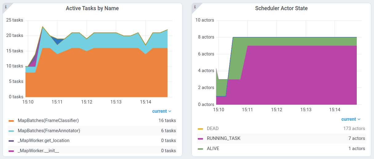Figure 8. View active tasks and actors for this job in the Ray Dashboard

We can also inspect hardware utilization in the Ray dashboard. We'll focus on the network activity. We can see two nodes receiving ~500MiB/s (these are the two GPU nodes hosting the FrameClassifier actors), and a number of other nodes driving significant traffic from 100-200MiB/s, likely sending data to the GPU nodes or between the decode and FrameAnnotator steps:

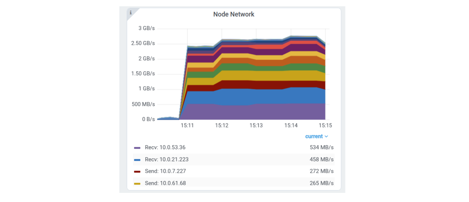Figure 9. Ray Dashboard showing network activity

The overall pipeline finishes in ~5 minutes, successfully processing ~350GB of video frame data total on a heterogeneous cluster of CPUs and GPUs. We see that Ray Data was able to pipeline the entire execution across the cluster to make the best use of memory.

LinkDiscussion

LinkOptimizations

In order to seamlessly execute such streaming topologies, Ray Data provides a number of optimizations under the hood. This includes:

Memory stability: Ray Data relies on the underlying Ray scheduler to schedule tasks and actors, but still needs to manage back-pressure across the streaming topology to bound memory usage and avoid object store spilling. It does this by only scheduling new tasks if it would keep the streaming execution under configured resources limits. Intuitively, enforcing a cap on intermediate result memory usage is needed to avoid degrading to bulk execution.

Data locality: While Ray will already place tasks on nodes where their input arguments are local, Ray Data's streaming backend extends this to optimize the scheduling of actor tasks. For example, in the above example, a lot of network traffic is avoided between the `decode_frames` and `FrameAnnotator` steps by routing decoded frames to actors that are on the same node.

Fault tolerance: Ray Data leverages Ray's built-in fault tolerance in order to handle object loss in large jobs. When objects are lost, they are recomputed based on their task lineage tracked by Ray. If actors were needed to produce these objects, Ray restarts these actors prior to re-submitting the task.

LinkScalability

To give an idea of the upper scalability envelope of Ray Data streaming, we ran a number of synthetic benchmarks that stressed Ray's object manager and Ray Data's streaming executor processing a 20TiB array dataset. Under the hood, Ray Data is using ray.remote() / ray.wait() to orchestrate the streaming topology, which means it is similarly scalable as Ray itself:

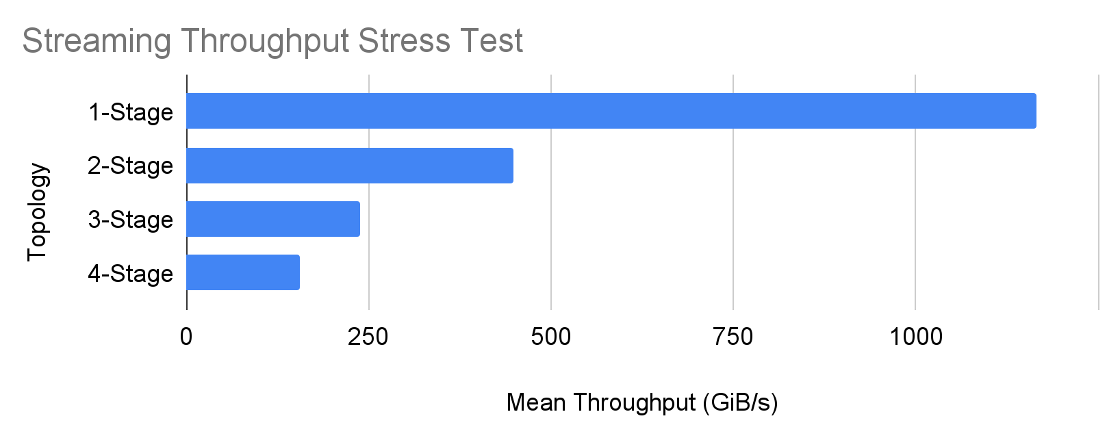Figure 10. Synthetic benchmarks stressing Ray's object manager and Ray Data's streaming executor processing a 20TiB array dataset

These benchmarks were run on a cluster of 500 machines, and test pipelines with between one to four stages similar to the video streaming example. We see that for the simplest pipeline on this cluster, Ray Data can process input data at a rate exceeding 1TiB/s. For more complex multi-stage pipelines, Ray Data can still sustain about 100-200GiB/s of end-to-end throughput on a large cluster.

LinkDistributed Training

A significant portion of Ray Train users today are also using Ray Data as a distributed data backend for ML training. Ray Data streaming allows these users to efficiently work with datasets that are larger than cluster memory for training, leveraging both CPU and GPU nodes to speed up their jobs. We are working on enhancing Ray Train's API to natively work with Ray Data streaming.

LinkWhat's next?

Today, early users are taking advantage of the Ray Data streaming backend to create efficient large-scale inference pipelines over unstructured data, including video and audio data. To learn more about how to build your own pipeline, check out the batch inference tutorial in our docs. We'll also be following up with a blog on more unstructured application examples. To learn more generally about streaming in Ray Data, check out the library docs, and let us know what improvements you'd like to see to Ray Data.

Also, we will be presenting at the Ray Summit. Register now — early bird registration is open until June 30, 2023.