Scaling Time Series Forecasting on Ray: ARIMA and Prophet on Ray

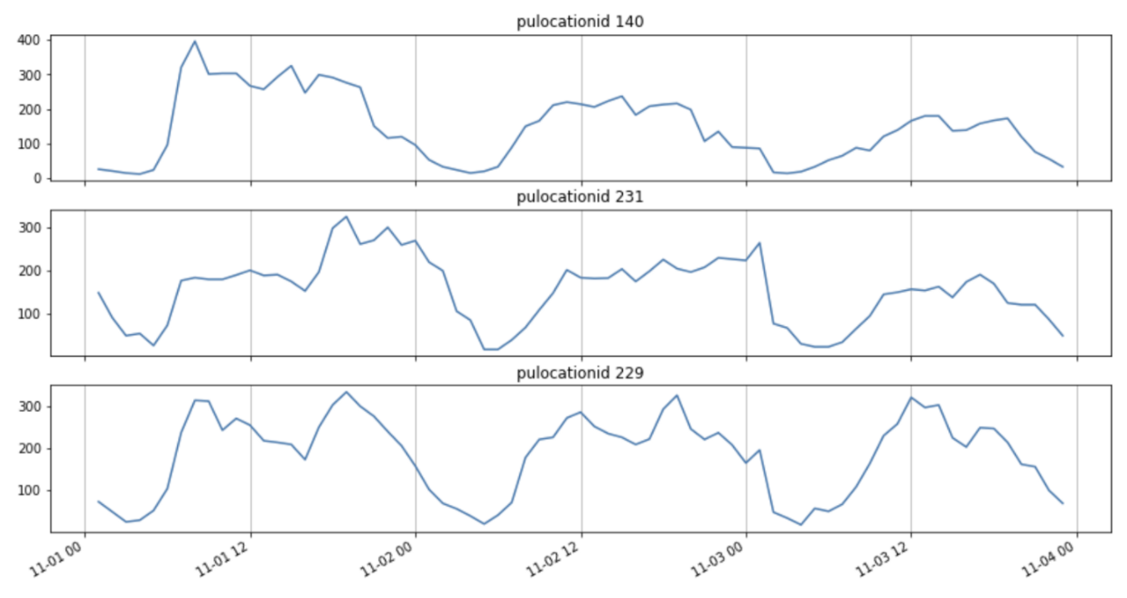
Image by Author. New York City Yellow Taxi ride volumes per location. 6 months of historical data were used in this blog.

Forecasting is an important part of running every business. You need to have an idea about what and how much to produce, especially if lead times are long, in order to have stock available for your customers. If you order too much, you’ll have excess inventory which carries cost. If you order too little, you might miss out on lost sales.

What if you’re a Data Scientist tasked with maintaining forecasts at a fast-growing company? You’re worried that the size of the data is increasing so fast that your models will have trouble keeping up. In today’s world, data drift is a given. Products, user features, and accompanying data are quickly changing. This means underlying statistical distributions of your input model features are also quickly changing. This means you need to re-train your models, possibly every week or more.

For the Data Scientist, training new models is not just about the time it takes to train that final model. Development time includes the time it takes to train all the candidate models, iterate on them, and select the best models. If it takes hours to train a single model, you won’t get your job done in time. You need to be able to iterate model training/inferencing faster. One way to iterate faster is to be able to parallelize your compute.

This blog will address the following topics:

• What is statistical forecasting?

• What is Ray and how does it distribute your Python model training and inferencing with ease?

• ARIMA on Ray

• Prophet on Ray

• What is Anyscale and how does it make it easy to run your Ray-distributed code on a cluster in the cloud?

LinkWhat is statistical forecasting?

Forecasting models generally fall into two categories: 1) local statistical models, and 2) global deep learning models.

“Local model” means each time series is trained one at a time, independently. That is, if you have 20K items to forecast, you need to train 20K statistical models. Each model has no knowledge of the other models.

“Global model” means each time series is an input, typically thought of as a neuron in a deep learning model, where behavior of all the inputs is learned as a global system. Intuitively this makes sense if there are dependencies between products, which can help improve accuracy of hard to forecast products.

This blog is about forecasting with local statistical models. The next blog will be about forecasting with global deep learning models.

LinkWhat is Ray?

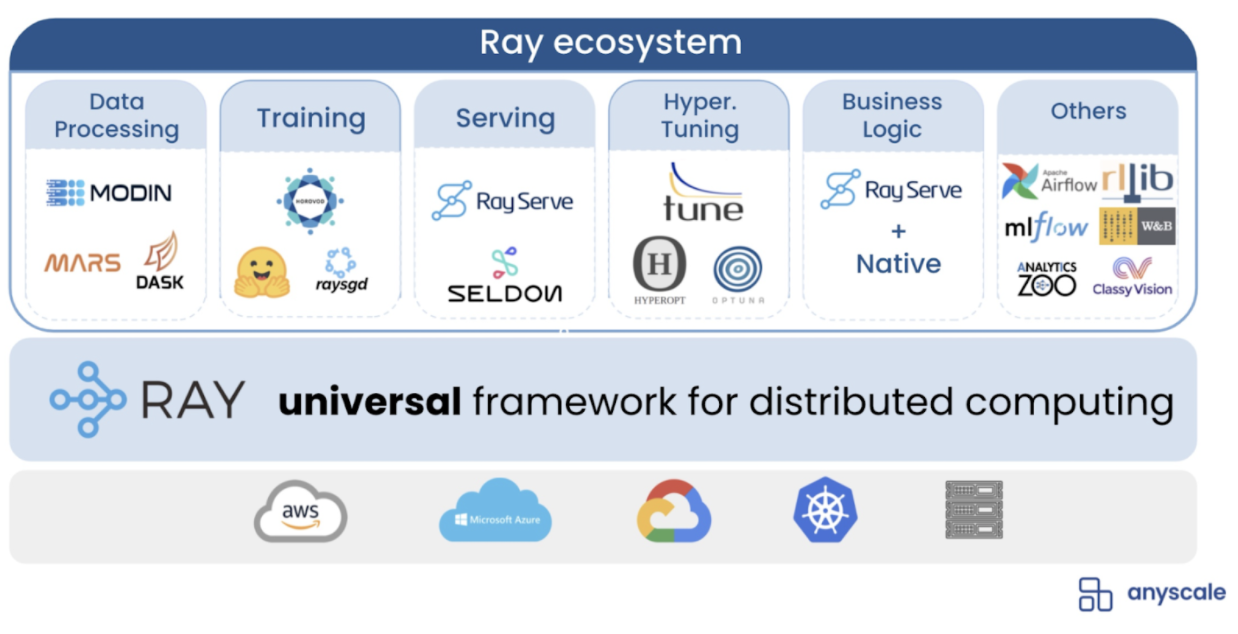
Ray is an open-source library developed at RISELab from UC Berkeley, which also developed Spark. Ray is the best practice parallelization engine behind Modin. Ray allows easy parallelization and distribution of existing Python code. Distributed Python code can then run on any type of cluster: a) your own laptop cores, b) AWS, GCP, or any common cloud.

Lots of Python ML code already exists in the world. Companies usually have a large in-house codebase developed for forecasting, including tricks learned over the years by domain experts, which work just for a given company’s data.

Today, distributing code is hard. It usually involves rewriting Python into multiprocessing Python or converting it to PySpark or SparkSQL. Ray makes it easy to take your existing Python code that runs sequentially and transform it into a distributed application with minimal code changes.  The resulting Ray-distributed code can run in parallel on underlying hardware.  See this blog about reducing 12 hour image processing runtime down to 4 minutes.  Also see this video demo of a recommendation system using xgboost with hyperparameter tuning on Anyscale.

Image from from Ion Stoica’s keynote at Ray Summit 2021. Ray and its ecosystem make it easy to to parallelize existing libraries like scikit-learn, XGBoost, LightGBM, PyTorch, TensorFlow, and much more.

LinkARIMA on Ray Example

Two of the most common time series statistical forecasting algorithms in use today are ARIMA and Prophet. At a high-level, ARIMA assumes causality between the past and the future. That is, the forecasted value at time t+1 has an underlying relationship with what happened in the past. You can think of ARIMA as building formulas. An ARIMA model consists of coordinates (p, d, q): p stands for the number of autoregressive terms, think of this as seasonality. d denotes the number of differences needed to make the time series stationary (i.e. have constant mean, variance, and autocorrelation). q represents the moving average portion or how many data points in the past will be exponentially smoothed to predict the future.

ARIMA models were originally developed in the R programming language and later converted to Python. One of the newer Python libraries is pmdarima, which implements auto.arima() from Rob Hyndman. 

All the sample code below uses Python 3.8 with Ray v1.8 and is available on github. To distribute ARIMA using Ray, follow Steps 1–4 below:

Step 1. Start a ray server locally. The idea here is you can test your distributed code locally. Iterate quickly and get all the bugs out. Before the added expense of testing the distributed code on a cloud. 

1
2
3
4
5
6
7
8
    # num_cpus, num_gpus are optional parameters
    # by default Ray will detect and use all available
    NUM_CPU = 8
    ray.init(
        # avoid error messages in case re-running this cell
        ignore_reinit_error=True, 
        num_cpus = NUM_CPU
    )    

Step 2. Convert the original ARIMA train function to a Ray function. Assume this is the original ARIMA train function.

1
2
3
4
5
6
7
8
9
10
11
12
13
14
15
16
17
18
19
    #add the Ray decorator
    @ray.remote(num_returns=3)
    def train_model_ARIMA_remote(
       theDF:pd.DataFrame, item_col:str,
       item_value:str, target_col:str,
       train_size:int=6,
    ) -> list:

       # split data into train/test
       train, test = train_test_split(
          theDF.loc[(theDF[item_col]==item_value), :],
          train_size=train_size
       )
       # train and fit auto.arima model
       model = pm.auto_arima(y=train[target_col])

       # return [train, test, model] 
       # here is the extra pickle step 
       return [train, test, pickle.dumps(model)]

Currently, ARIMA requires an extra pickle step to ensure statsmodels library objects are serialized correctly (explanation). The extra pickling/unpickling is for portability. Since the code behind the scenes will be distributed, the objects need to be compatible with pickle.HIGHEST_PROTOCOL so they can run anywhere on any node, and be retrieved again. Ray might eliminate the need for the pickle work-around in the future.

Steps to convert the ARIMA train function:
a) Add the ray decorator, specifying 3 return outputs.
b) Add an extra pickle step

Below is the ray version of the ARIMA train function.

1
2
3
4
5
6
7
8
9
10
11
12
13
14
15
16
17
18
#add the Ray decorator
@ray.remote(num_returns=3)  
def train_model_ARIMA_remote(
                theDF:pd.DataFrame, item_col:str
                , item_value:str, target_col:str
                , train_size:int=6) -> list:

# split data into train/test
    train, test = train_test_split(
         theDF.loc[(theDF[item_col]==item_value), :]
         , train_size=train_size)

    # train and fit auto.arima model
    model = pm.auto_arima(y=train[target_col])

    # return [train, test, model]     
    # here is the extra pickle step
    return [train, test, pickle.dumps(model)]

Step 3. Convert the original ARIMA inference function to a Ray function.
Assume this is the original ARIMA inference function.

1
2
3
4
5
6
7
8
9
10
11
12
13
14
15
    def inference_model_ARIMA(
       model:"pmdarima.arima.arima.ARIMA",
       test:pd.DataFrame,
       item_col:str,
       target_col:str,
    ) -> pd.DataFrame:

       # inference on test data
       forecast = pd.DataFrame(
           model.predict(
               n_periods=test.shape[0], 
               index=test.index,
           )
       )
       return forecast

Steps to convert the ARIMA inference function:
a) Add the ray decorator.  This time we don’t need extra options on the Ray decorator, which by default returns 1 object.
b) Change the type of model object being passed to just bytes
c) Add an extra unpickle step

Below is the Ray version of ARIMA inference.

1
2
3
4
5
6
7
8
9
10
11
12
13
14
15
16
17
18
19
    @ray.remote
    def inference_model_ARIMA_remote(
       model_pickle:bytes,
       test:pd.DataFrame,
       item_col:str,
       target_col:str,
    ) -> pd.DataFrame:

       # Here is extra unpickle step
       model = pickle.loads(model_pickle)

       # inference on test data
       forecast = pd.DataFrame(
           model.predict(
               n_periods=test.shape[0], 
               index=test.index,
           )
       )
       return forecast

Step 4. Instead of calling the original train and inference functions, now call the distributed functions.
Assume this is how originally the ARIMA train and inference functions were called.

1
2
3
4
5
6
7
8
9
10
11
12
13
14
15
16
17
18
19
20
21
22
23
24
25
26
27
28
29
30
31
    model = []
    train = []
    test = []

    # Train every model
    train, test, model = map(
    list,
    zip(
       *(
          [
             train_model_ARIMA(
                g_month.set_index("time"),
                item_col="pulocationid",
                item_value=v,
                target_col="trip_quantity",
                train_size=6,
             )
             for p, v in enumerate(item_list)
          ]
       )
      ),
    )

    # Inference every model
    forecast = [
       inference_model_ARIMA(
          model[p], test[p], item_col="pulocationid", 
          target_col="trip_quantity"
       )
       for p in range(len(item_list))
    ]

Ray does parallel remote compute until you request objects. Ray remote compute, or Python “futures”, are not “lazy” as in spark processing.  The .remote() calls are made in parallel asynchronously.  Values are retrieved sometime in the future using ray.get().  At this point, all the distributed code executions are gathered and given back to the user. Behind the scenes, ray object references are converted back to pandas dataframes, or whatever type of object was requested by the user.

Steps to convert the ARIMA training and inference calling functions:
a) Call the Ray-parallelized functions with the .remote() method
b) Get the forecasts using ray.get()

Below is the Ray version of calling ARIMA train and inference functions in Python.

1
2
3
4
5
6
7
8
9
10
11
12
13
14
15
16
17
18
19
20
21
22
23
24
25
26
27
28
29
30
31
32
33
34
35
36
    model = []
    train = []
    test = []

    # Train every model
    train, test, model = map(
    list,
    zip(
         *(
             [  
                # call Ray functions using .remote() method
                train_model_ARIMA_remote.remote(
                   g_month.set_index("time"),
                   item_col="pulocationid",
                   item_value=v,
                   target_col="trip_quantity",
                   train_size=6,
                )
                for p, v in enumerate(item_list)
             ]
          )
       ),
    )  

    # Inference every model
    forecast_obj_refs = [ 
       # call Ray functions using .remote() method
       inference_model_ARIMA_remote.remote(
          model[p], test[p], item_col="pulocationid", 
          target_col="trip_quantity"
       )
       for p in range(len(item_list))
    ]

    # ray.get() means block until all objectIDs are available 
    forecast = ray.get(forecast_obj_refs)

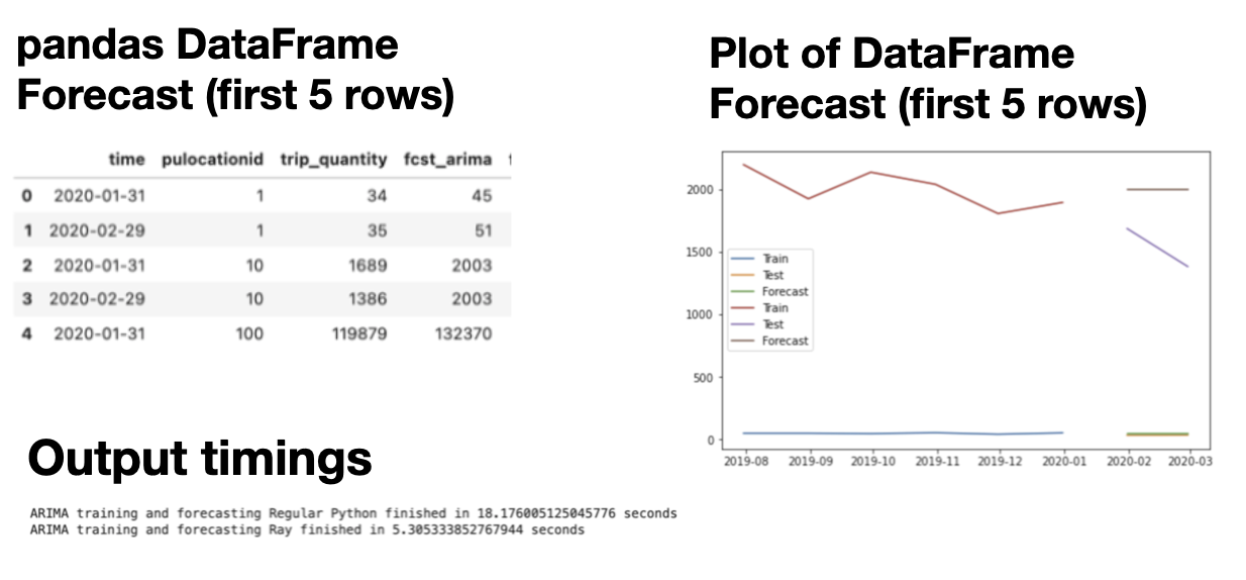
That’s it! You’ve just distributed ARIMA training and inferencing using Ray!  All items in the item_list will be processed in parallel now.  Sample output is shown below.

Only displaying 2 forecasts, instead of all the forecasts.

LinkProphet on Ray Example

Prophet is a special case of the Generalized Additive Model. Whereas ARIMA tries to build a formula for future values as a function of past values,  Prophet tries to detect “change points”; you can think of Prophet as curve-fitting.  

The newest open-source library from Facebook, Kats, includes the original Prophet plus newer libraries for Multivariate forecasting, DeepLearning forecasting, and Anomaly Detection. A closer inspection of the githubs shows that the Prophet inside Kats is maintained more recently than the original Prophet.

All the sample code below uses Python 3.8 with Ray v1.8 and is available on github. To distribute Prophet using Ray, follow Steps 1–4 below:

Step 1. Start a ray server locally and tell it how many processors it can use. See the ARIMA example above.

Step 2. Nothing! No need to change the original train and inference Prophet functions.

Step 3. Add a Ray decorator to your existing train and inference functions. Decorators can be added manually by copy/pasting/modifying def function code, as we showed in the ARIMA example above. Decorators can also be added declaratively, as shown below, which is easier when you do not need to modify original code.  Decorators can be added manually by copy/pasting/modifying def function code, as we showed in the ARIMA example above. Decorators can also be added declaratively, as shown below, which is easier when you do not need to modify original code.

1
2
3
4
# Convert your functions to ray parallelized functions
train_model_PROPHET_remote = 
     ray.remote(train_model_PROPHET).options(num_returns=3) 
inference_model_PROPHET_remote = ray.remote(inference_model_PROPHET)

Step 4. Instead of calling the original train and inference functions, now call the distributed functions.
Assume this is how originally the Prophet train and inference functions were called.

1
2
3
4
5
6
7
8
9
10
11
12
13
14
15
16
17
18
19
20
    train = []
    test = []
    model = []
    forecast = []

    # Train every model
    train, test, model = map(list, zip(*(
       [train_model_PROPHET(g_month,
          item_col='pulocationid',
          item_value=v,
          target_col='trip_quantity',
          train_size=6),
       for p,v in enumerate(item_list)] )))

    # Inference every model
    forecast = [inference_model_PROPHET(model[p],
                  test[p],
                  item_col='pulocationid',
                  target_col='trip_quantity') 
               for p in range(len(item_list))]

Steps to convert the Prophet training and inference calling functions:

a) Call the Ray-parallelized functions with the .remote() method
b) Get the forecasts using ray.get().

Below is the Ray version of calling Prophet train and inference functions in Python.  For clarity below, I renamed train, test, model, and forecast variable names, but it is  not required.

1
2
3
4
5
6
7
8
9
10
11
12
13
14
15
16
17
18
19
20
21
22
23
    train_obj_refs = []
    test_obj_refs = []
    model_obj_refs = []
    forecast_obj_refs = []

    # Train every model
    train_obj_refs, test_obj_refs, model_obj_refs = map(list, zip(*(
       [train_model_PROPHET(g_month,
          item_col='pulocationid',
          item_value=v,
          target_col='trip_quantity',
          train_size=6),
       for p,v in enumerate(item_list)] )))

    # Inference every model
    forecast = [inference_model_PROPHET(model_obj_refs[p],
                  test_obj_refs[p],
                  item_col='pulocationid',
                  target_col='trip_quantity') 
               for p in range(len(item_list))]

    # ray blocking step, to get the forecasts
    forecast_prophet = ray.get(forecast_obj_refs)

That’s it! You’ve just distributed Prophet training and inferencing using Ray!

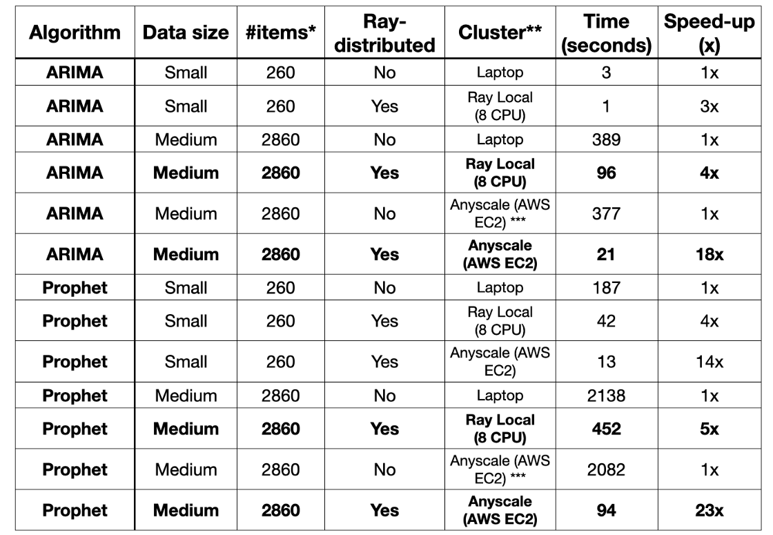
These small tweaks decreased runtimes for Prophet by 4x on a laptop. That is, a speed-up of 300%. See table at end of this article for more runtimes

Note: We observed more speed-up for Prophet since it is longer-running than ARIMA. Both ARIMA and Prophet, as “statistical models”, take very small data inputs, so we would expect correspondingly-sized speed-ups from distributing code. In contrast, deep-learning models require large data inputs and long-running training times; we will expect to see larger speed-up effects.

LinkWhat is Anyscale?

Once you’ve debugged and tested your newly-distributed Python code using Ray locally on local cores, you’re ready to run that same code in the cloud.

Anyscale simplifies building, running and managing Ray applications, spins up compute in the cloud, runs your code distributed in-parallel across clusters, uses built-in rules for autoscaling, and is compatible with all commonly used cloud providers (AWS, GCP, ...). Anyscale is suitable for a multi-cloud strategy as its use does not create any vendor lock-in. Anyscale only depends on basic compute instances, which makes it less expensive to operate than many packaged offerings sold as services.

Note: Currently Anyscale is available through invite-only private Beta.  Sign up here to try it out.  

Below is a quick, 3-step guide to getting started with Anyscale. For more details, see “Get Started”. Anyscale is available from a web UI Console (screenshots below) or client API . Behind the scenes, Anyscale uses open-source Ray.

Step 1. Authenticate into the cloud through your Anyscale account. You only need to do this once.

• Open the console to https://console.anyscale.com/credentials

• Copy the create json file command

• Paste it in your local terminal.

Step 2. Run ray.init() from within your application.

Comment out the previous ray init(), which ran ray server locally.
# NUM_CPU = 8
# ray.init( ignore_reinit_error=True , num_cpus = NUM_CPU)

Add in a new ray.init() to connect to the cluster. 

You can specify more pip installs, clone a github repo, or copy a whole code directory into either the cluster or runtime environments.  The cluster config is used first, then the runtime config, if specified, will override the cluster config.  The result of the configs is to install additional libraries, code, and data on every node of the cloud cluster automatically.  

Below, I’m using a default cluster config (which specifies autoscaling policies), and I’m putting the extra pip install in the runtime config.  The my_cluster_name in the url string “anyscale://my_cluster_name” will become your new cluster name.

my_env={"working_dir": ".", "pip": ["pmdarima", "kats"]}
ray.init("anyscale://my_cluster_name", runtime_env=my_env)

Step 3. Run your python code (or notebook) the way you would normally. It will automatically run in parallel and distributed across clusters in the cloud!

While your application is running, you can monitor your cluster usage in the Anyscale console under Clusters.

Below is a table summarizing all the runtimes. Notice that un-parallelized Python code does not speed up, even if running it in a typical cloud.

* #items means number of line items or number of distinct time series to forecast. ** Laptop was a macbook pro (13-inch, M1, 2020). Anyscale settings on AWS were: Head node type m5.2xlarge, Worker nodes m5.4xlarge and g4dn.4xlarge, Autoscaling turned on up to max 10. *** Regular Python (not Ray-distributed code) running in the cloud runs on 1 CPU (Head node) only.

LinkConclusion

This post presented how a data scientist can scale the training and inference of their ARIMA and Prophet models.  We showed how you can easily parallelize and distribute Python code, without re-writing the underlying, existing codebase.

The Ray distributed Python code was

1. Distributed and executed in parallel across local laptop cores by a local Ray server.

2. Distributed and executed in parallel, in a cloud, by Anyscale cluster management.

Some readers may be wondering, can these patterns for easily distributing Time Series Forecasting model training and inference, also be used for distributing ANY large data inputs and ANY AI/ML algorithms? We think the answer is Yes! 

Part 2 in this series of Faster Forecasting will be about parallelizing large deep learning models.