Practical tips for training Deep Q Networks

This series on reinforcement learning was guest-authored by Misha Laskin while he was at UC Berkeley. Misha's focus areas are unsupervised learning and reinforcement learning.

In the previous entry in this series, we covered Q learning and wrote the Deep Q Network (DQN) algorithm in pseudocode. While DQNs work in principle, in practice implementing RL algorithms without understanding their limitations can lead to instability and poor training results. In this post, we will cover two important limitations that can make Q learning unstable as well as practical solutions for resolving these issues.

Recall that the Bellman equation relates the Q function for the current and next timestep recursively:

DQNs use neural networks to estimate both and and minimize the mean squared error (MSE) between the two sides of this equation. This brings us to the first problem.

LinkProblem 1: The Bellman error as a moving target

The Bellman error is just the MSE between the two sides of the Bellman equation. Let’s write down the definition of mean squared error: where is the prediction and is the target value. In supervised regression problems, is a fixed true value. Whenever we make a prediction we don’t have to worry about the true value changing.

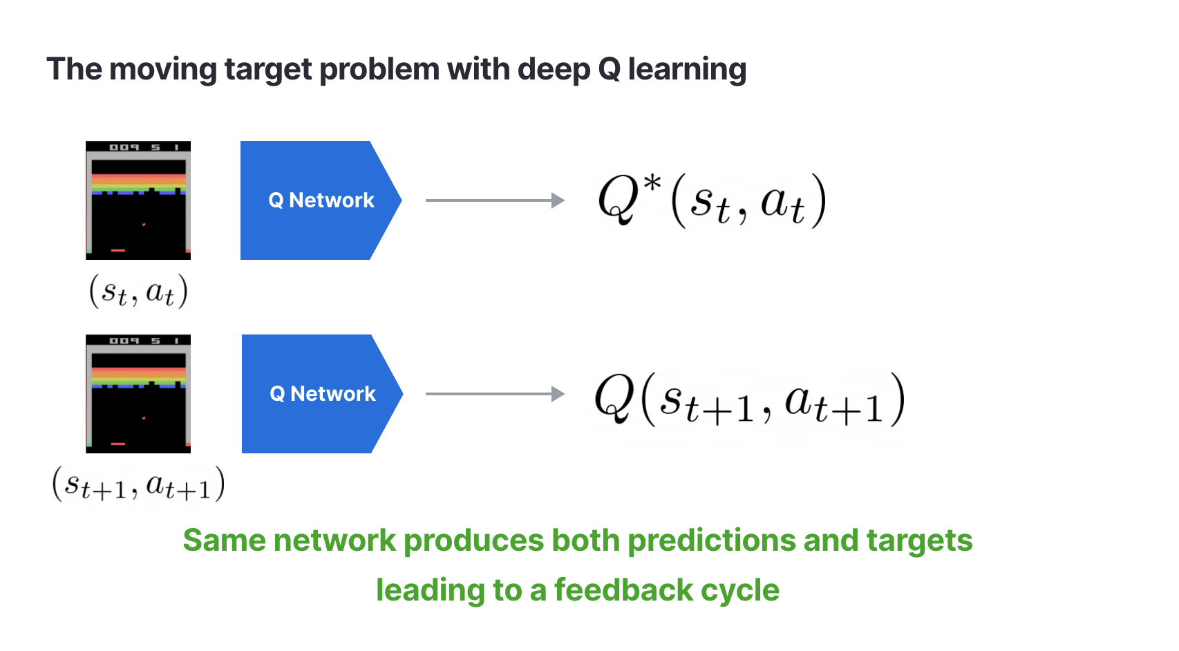
However, in Q learning and meaning that the target is not the true underlying value but is also a prediction. Since the same network is predicting both and this can cause a runaway loss. As changes so will the prediction for leading to a feedback cycle.

LinkSolution 1: Keep a slowly updating target network

A practical solution to this problem is to use two different but similar networks to predict and to stabilize training. The original DQN uses the Q network to predict and keeps an old copy of the Q network, which it updates after a fixed training interval, to predict the target . This ensures that the targets stay still for fixed periods of time. A drawback of this solution is that the target values change suddenly several times during training.

Another solution used in a subsequent paper from DeepMind (Lillicrap et al. 2015) is to maintain a target network whose weights are an exponentially moving average (EMA) of the prediction network. EMA weights change slowly but smoothly which prevents sudden jumps in target Q values. The EMA strategy is used in many state-of-the-art RL pipelines today. In code it looks like this:

1
2
3
4
5
6
7
"""
Exponentially moving average
"""
def target_Q_update(pred_net, target_net, beta=0.99):
	target_net.weights = beta * target_net.weights + \
												(1-beta) pred_net.weights
	return target_net

LinkProblem 2: Q learning is too optimistic

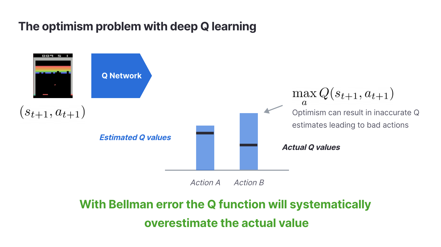
Moving targets are not the only issue with Q learning. Another problem is that predictions made with Q functions optimized via the Bellman error are too optimistic. Although optimism is viewed favorably among people, it can easily derail an RL system from being useful. From the RL perspective, optimism means the algorithm is overestimating how much return it will get in the future. If you’re a business relying on RL to make mission critical decisions, this means trouble.

So where does optimism in Q learning come from? As with the moving target problem, it comes straight from the Bellman equation. At the start of training, the neural network does not know the real Q value accurately so when it makes a prediction, there is some error. The culprit is the max operation. The target prediction will always choose the highest valued Q even if it was incorrect. To make this point clearer, we provide an example:

From this example, you can see that when in doubt the target Q function will always be optimistic. The issue is that this optimism is systematic, meaning that the DQN will make more errors from optimistic estimates than it will from pessimistic ones due to the operation. This optimistic bias will quickly compound during training.

LinkSolution 2: Train two Q networks and use the more pessimistic one

Double Q networks address this problem by training two totally different and independent Q functions. To compute the target network, Double DQNs select the minimum value from the estimates of the two Q functions. You can think of the two Q networks as an ensemble. Each network votes on what it thinks is and the most pessimistic one wins. In principle, you could have N such networks to get more votes, but in practice two is enough to resolve the optimism problem. Here’s how a double Q target calculation looks like in code:

1
2
3
def compute_target_Q(target_net1, target_net2):
	target_Q = minimum(target_net1, target_net2, dim=1)
	return target_Q

When run on Atari, double Q learning results in much more conservative estimates of the Q function than DQNs.

Value estimates in Atari for DQNs and Double DQNs. While DQNs overestimate the value, Double DQNs are much more conservative. Source: https://arxiv.org/abs/1509.06461

LinkConclusion

We’ve discussed two challenges when training Q networks as well as their solutions. This is just a small taste of the different issues that may be encountered when training RL algorithms. Luckily, understanding these issues from first principles allows you to form intuition for RL systems and develop practical solutions to get your algorithms to work.

If you're interested in exploring more about RL, check out the resources below:

• Register for the upcoming Production RL Summit, a free virtual event that brings together ML engineers, data scientists, and researchers pioneering the use of RL to solve real-world business problems

• Learn more about RLlib: industry-grade reinforcement learning

• Check out our introduction to reinforcement learning with OpenAI Gym, RLlib, and Google Colab

• Get an overview of some of the best reinforcement learning talks presented at Ray Summit 2021