A distributed shuffle is a data-intensive operation that usually calls for a system built specifically for that purpose. In this blog post, we’ll show how a distributed shuffle can be expressed in just a few lines of Python using Ray, a general-purpose framework whose core API contains no shuffle operations.

Shuffling a small dataset is simple enough to do in memory. However, a larger dataset brings new challenges such as:

1. Multiple nodes, to scale memory capacity past a single machine and to enable parallel processing within the map and reduce phases.

2. Spilling to external storage, when the total dataset is larger than the cluster’s total memory capacity.

3. Enforcing memory limits, to avoid triggering expensive out-of-memory handling by the OS, such as swapping to disk or triggering the out-of-memory (OOM) killer.

In an earlier blog post, we showed how Ray can be used as a common substrate for data processing applications. Here, we’ll do a deep dive into how Ray executes an out-of-core distributed shuffle expressed as tasks in Python.

LinkWhat is a shuffle?

Because of its size, a distributed dataset is usually stored in partitions, with each partition holding a group of rows. This also improves parallelism for operations like a map or filter. A shuffle is any operation over a dataset that requires redistributing data across its partitions. Examples include sorting and grouping by key.

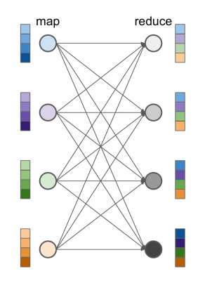
A common method for shuffling a large dataset is to split the execution into a map and a reduce phase. The data is then shuffled between the map and reduce tasks. For example, suppose we want to sort a dataset with 4 partitions. The goal is to produce another dataset with 4 partitions, but this time sorted by key.

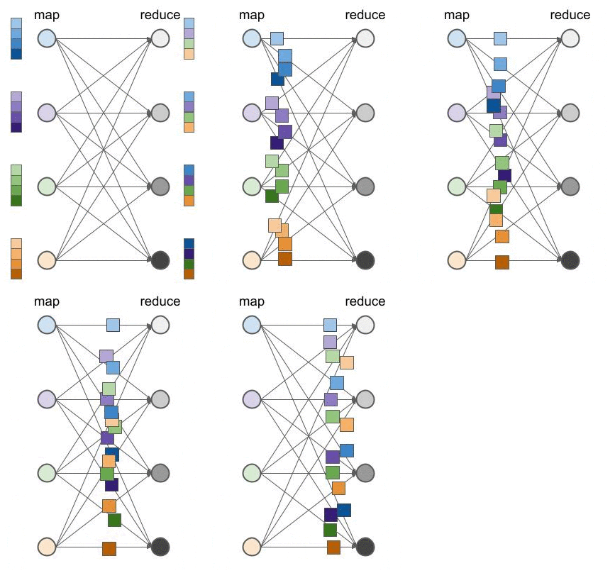Shuffling a distributed dataset with 4 partitions, where each partition is a group of 4 blocks. In a sort operation, for example, each square is a sorted subpartition with keys in a distinct range. Each reduce task then merge-sorts subpartitions of the same shade.

The above diagram shows this process. Initially, the unsorted dataset is grouped by color (blue, purple, green, orange). The goal of the shuffle is to regroup the blocks by shade (light to dark). This regrouping requires an all-to-all communication: each map task (a colored circle) produces one intermediate output (a square) for each shade, and these intermediate outputs are shuffled to their respective reduce task (a gray circle).

This sort of program can be written with Ray using Python functions. A task is created by invoking the function. Each map task returns multiple values, one per reduce task, and each reduce task takes these outputs as its arguments. A sort would then look something like this using the Ray API:

1import ray
2import numpy as np
3
4@ray.remote
5def map(data, npartitions):
6    outputs = [list() for _ in range(npartitions)]
7    for row in data:
8        outputs[int(row * npartitions)].append(row)
9    return tuple(sorted(output) for output in outputs)
10
11@ray.remote
12def reduce(*partitions):
13    # Flatten and sort the partitions.
14    return sorted(row for partition in partitions for row in partition)
15
16ray.init()
17npartitions = 4
18dataset = [np.random.rand(100) for _ in range(npartitions)]  # Random floats from the range [0, 1).
19map_outputs = [
20        map.options(num_returns=npartitions).remote(partition, npartitions)
21        for partition in dataset]
22outputs = []
23for i in range(npartitions):
24    # Gather one output from each map task.
25    outputs.append(reduce.remote(*[partition[i] for partition in map_outputs]))
26print(ray.get(outputs))

LinkSingle-node shuffle, when memory is not a constraint

A distributed shuffle is challenging because of the all-to-all dependencies between the map and reduce phase. With N partitions, this leads to N^2 intermediate outputs that must be shuffled between the map and reduce tasks.

But when the data all fits in memory, this is simple enough to do. Let’s take a look at how this works on Ray with a smaller version of the previous example.

We want to execute this graph over a 4GB dataset and 2 partitions. Then, each intermediate output (squares) will be 1GB:

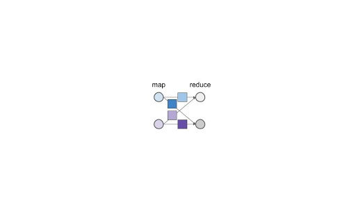
Let’s try it on this machine with 2 CPUs and 8GB RAM:

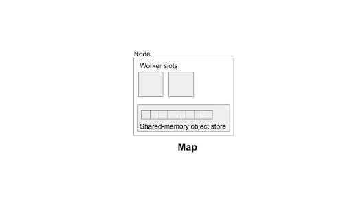
First, Ray schedules the map tasks (blue and purple) onto the two worker slots. These execute in parallel and create their objects (blue and purple squares) in the local Ray object store.

Next, Ray schedules the reduce tasks (gray circles). Ray resolves the reduce tasks’ dependencies by only scheduling a reduce task once all of its arguments (the blue and purple squares produced by the map phase) are local. Each worker gets a copy of the map outputs from the local object store. Since the object store is implemented with shared memory, this can be done with zero copies if the objects are based on NumPy. Once the reduce tasks finish, Ray automatically garbage-collects their arguments.

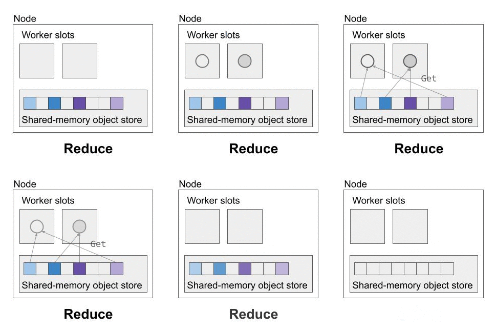
Ray manages the parallelism and task dependencies for this small shuffle, but of course it’s pretty straightforward because all of the data fits in the memory of a single machine. In the next example, we’ll take on the full-sized shuffle and on multiple nodes.

LinkMulti-node shuffle, with spilling to external storage

Let’s try a larger example, say 16GB with 4 partitions with intermediate outputs (squares) of 1GB:

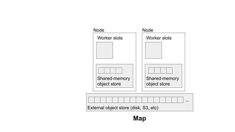
Now we want to execute it in a distributed, out-of-core setting, say with a cluster of 2 machines, each with 1 CPU and 4GB memory. We’ll also add an external storage system since we can’t fit the entire dataset in memory:

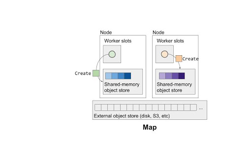
Since we can only execute two tasks at a time, we’ll have to schedule each phase in two waves. The first wave of the blue and purple map tasks looks pretty much the same as in the single-node case, since we have enough memory to store their outputs:

But what happens when the other two map tasks (green and orange) are run? We don’t have enough memory to store those outputs!

At this point, each Ray node begins to spill its current objects (blue and purple) to external storage to make room for the new objects (green and orange). We need to spill the objects instead of deleting them since the reduce tasks still depend on them.

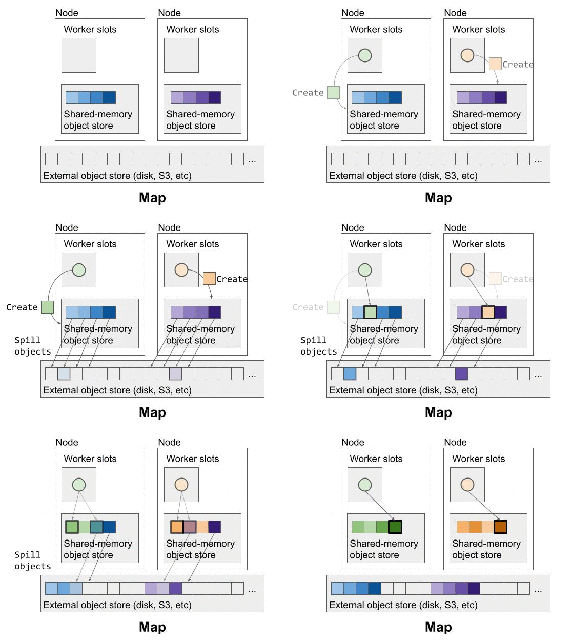The blue and purple objects are automatically spilled to remote storage to make room for new map task outputs (green and orange).

Of course, during the reduce phase, we also have to restore the spilled objects so that the reduce workers can fetch them from memory. Each Ray node will determine which objects to restore based on the dependencies of the scheduled tasks, outlined in red below. To make room for the reduce tasks’ arguments, each Ray node again spills any local objects.

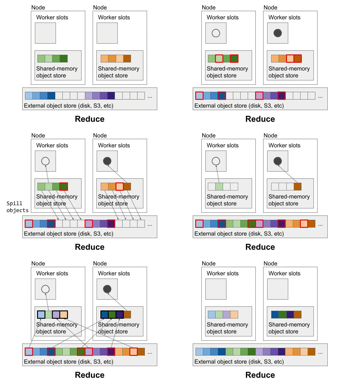Restoring spilled objects that are now needed by the reduce tasks. Squares outlined in red are the objects needed by the two scheduled reduce tasks (gray circles). To make room for the task arguments, Ray spills again, this time spilling the green and orange map outputs.

In total, this workload required one round of spilling and restoring the N^2 intermediate outputs produced by the map tasks, not including the memory needed to read the initial dataset and write the final result. For example, with a 16GB dataset, each intermediate output would be 1GB and we would write and read 16GB of data to and from external storage during the shuffle step.

When the partitions are smaller, we may be limited by the external storage system’s random IO capacity. Too many small read and write requests can cause external storage to become a bottleneck. To avoid this, Ray also batches multiple intermediate outputs to the same write request (e.g., a file). Reads are trickier to combine, but we plan to implement optimizations from the literature here in the future.

LinkLimiting memory while preventing deadlock

In the previous two examples, we always had enough memory to execute as many tasks as there were cores. In the 2-node example, we had 1 CPU and 4GB of memory on each node. Since this was exactly the amount that we needed to execute one task, scheduling was straightforward.

However, the resources won’t always be so well-balanced. One challenge in memory-intensive workloads is achieving parallelism without running out of memory. We want to execute tasks in parallel, up to the number of cores on a machine, but we also don’t want to execute so many tasks in parallel that they exceed the memory capacity of the node. Doing so could trigger the OS’s out-of-memory handling, such as the OOM killer.

Ray avoids this by enforcing a limit on the total memory used by each node’s object store, which can be configured by the user. However, this is only part of the solution. If we try to schedule based only on CPU availability, and ignore memory requirements, we could easily run into a deadlock.

For example, let’s say we want to execute the previous example on a single machine with 2 CPUs and 6GB memory. If we schedule tasks based on CPU availability, we could cause a deadlock like this:

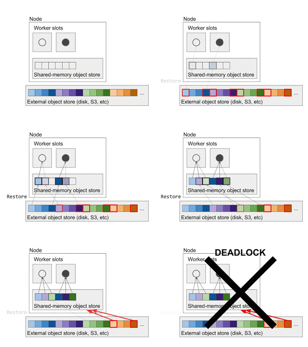Example of a possible deadlock with naive scheduling that considers only CPU availability. The scheduler tries to schedule both reduce tasks (gray circles) at once, causing a deadlock because both tasks require one more block of memory to run.

A task can only start once all of its dependencies are in the local object store. That means that to execute two reduce tasks in parallel, we would need 8GB of memory total to store their combined arguments. But we only have 6GB in this case, so we end up with a deadlock. Neither task can release its arguments until it finishes, but each of them requires an additional 1GB of memory to start execution.

To prevent this issue, Ray’s scheduler also takes into account the memory requirements for each task, computed from the size of its input arguments. Then, the system schedules tasks based on the total CPU and memory availability of the node:

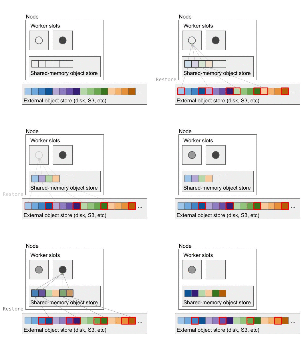Ray prevents the deadlock by scheduling tasks based on CPU and memory availability. Ray sees that there is only enough memory to execute one task at a time, so it fetches the arguments for the light gray task first. Once that task finishes, it then repeats for the dark gray task, and so on.

So in this example, Ray will see that each task needs 4GB of memory total to store its arguments. Since we only have 6GB of memory, Ray will only fetch the arguments for one of the reduce tasks at a time, even though we have enough CPUs to execute two at a time. Once one reduce task finishes, we can free its arguments and repeat for the next reduce task in the queue.

LinkConclusion

In this blog post, we showed how Ray provides memory management for data-intensive applications. To do so, Ray:

1. Provides a high-performance shared-memory object store.

2. Spills objects transparently to external storage once memory is full.

3. Applies admission control during task scheduling to enforce memory limits and prevent deadlock.

In our next blog post on data processing, we’ll discuss some of the challenges in scaling up this design to sort 100TB. If you're interested in helping us improve Ray and its user experience, we're hiring for Ray core and platform.