Reinventing Multi-Modal Search with Anyscale and MongoDB
LinkSummary
In this guide, we will walk through a comprehensive solution for improving a legacy search system over multi-modal data using Anyscale and MongoDB. We will showcase how to build:
📈 A scalable, multi-modal data indexing pipeline that performs complex tasks like:
Multi-modal model batch inference
Vector embedding generation
Inserting data into a search index
Delta refreshes of the search index
🔍 A performant hybrid search backend that:
Self hosts embedding models
Combines lexical text matching with semantic search querying.
🖥️ A simple user interface for interacting with the search backend.
We will be making use of:
MongoDB cloud as the central data repository for:
Enabling vector search across multiple fields and dimensions via MongoDB Atlas Vector Search.
Being a ubiquitous choice in the space for its flexibility and scalability.
Supporting the storage of multi-modal data like images, text, and structured data.
Anyscale platform as the AI compute platform for:
Running performant batch inference compute jobs.
Enabling highly available and scalable deployments.
Optimally scaling and utilizing costly compute resources.
LinkThe Problem with Legacy Search Systems
Enterprises that deal with a large volume of multi-modal data often require a performant and robust search system. However, traditional search systems have certain limitations that need to be addressed:
Inadequate support for unstructured data:
Legacy search systems typically only offer lexical matching for text data, while unstructured data from other modalities, such as images, remains unsearchable.
Dependence on data quality and relevance:
If certain metadata fields are missing or of poor quality, the search system will be unable to effectively utilize them. In small datasets, these metadata issues might be easily fixed, but given the scale of enterprise datasets, manual curation and improvement is generally not an option.
To overcome these limitations, we will make use of generative and embedding models to enrich and encode the data, enabling a more sophisticated search experience.
LinkUse Case: Improving Search for an E-commerce Platform
In our example, we will tackle the following use case: An e-commerce platform that has a large catalog of products and would like to improve its search relevance and experience.
The dataset we will be using is the myntra dataset which contains images and metadata of products for Myntra, an Indian fashion e-commerce company. The goal is to improve the search capabilities of the platform by implementing a scalable multi-modal search system that can handle both text and image data.
The legacy search system only allows for:
Lexical search against the product name
Matching on the product price and rating
For instance, performing a search for a “green dress” will yield back items whose product name matches on the term “green” or “dress” (we used standard lexical search from MongoDB Atlas which converts the text to lowercase and splits it based on word boundaries to create separate tokens to match on—search results are ranked using a BM25 score.)
Below is a screenshot showcasing the results returned from the “green dress” query. Note how the shown product names either contain the token “green” or “dress” in them (primarily “green” in the shown screenshot).

Because of the legacy search system’s limitations, the matched results contain items that are not relevant to the users’ query and intent, such as “Bio Green Apple Shampoo.” The existing lexical search precision is constrained by the quality of the provided product name and will still suffer from poor recall of items that do not contain relevant information in their product name.
LinkSolution: Improving Search with Anyscale and MongoDB
On a high level, our solution will consist of:
Using Anyscale to run multi-modal large language models (LLMs) and generate product descriptions from the provided product image and name.
Using Anyscale to run large-language models and generate product metadata fields that are useful for search.
Using Anyscale to run embedding models for encoding the product names and generated descriptions, and indexing the resulting numeric vectors into a vector search engine like MongoDB Atlas Vector Search.
Below is a screenshot showcasing the results returned from the “green dress” query after improving our search engine. Notice how the shown products are more relevant to the users’ query and intent thanks to the semantic search capabilities of the new system. The new system uses images to enrich the semantic meaning of the product name, which improves the search capabilities. For instance, the system is able to fetch relevant items that do not contain the token “green” in their product name but that are indeed green dresses.

Additionally, on the left, we can see AI-generated metadata filters that can be used to further refine the search results. For the same query “green dress,” we can further filter the results by metadata fields such as “category,” “season,” and “color” to strictly match on filters like “color=green”, “category=dress”, and season=“summer or spring.”

LinkA discussion on alternative approaches to search over multi-modal data
Note that an alternative approach to encoding images is by making use of multi-modal embedding models like CLIP. To learn more about this approach, view our blog post on cross-modal search for e-commerce. This approach might be less computationally intensive than using a generative model like LLaVA, but it doesn’t allow for conditioning the generated semantic meaning of the image with the product name. For instance, a photo of a model wearing many items of clothing or against a background of other items might have its semantic signal dissipated across all the items in the photo, making it far less useful (see the image of “Girls Embellished Net Maxi Dress” in the screenshot above with the child model talking on the phone as an example).
LinkSystem-level Architecture
We split our system into an offline data indexing stage and an online search stage. The data indexing stage needs to be run periodically whenever new data is added to the system, while the search stage is an online service that handles search requests.
LinkData Indexing Stage
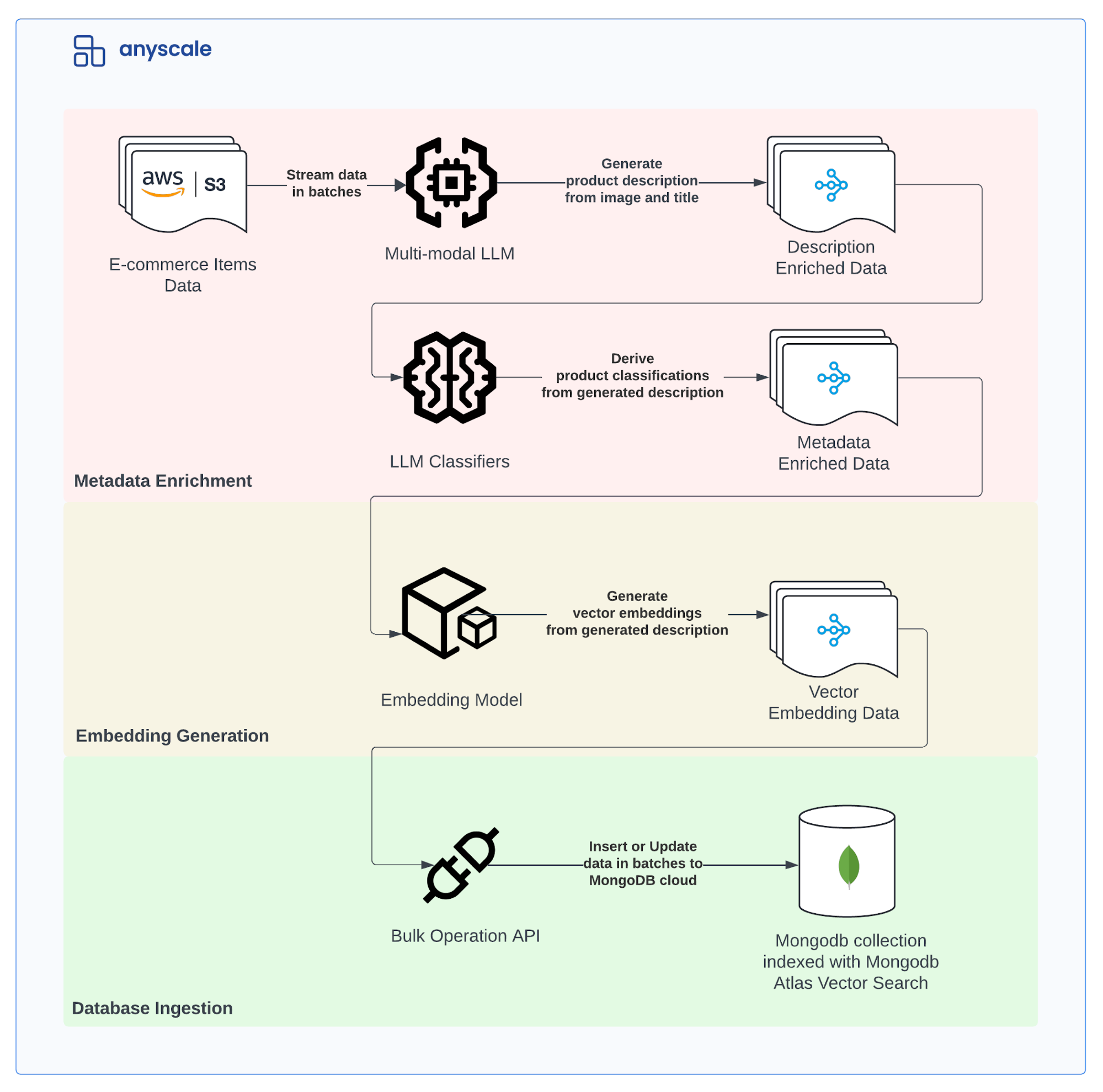
The indexing stage is responsible for processing, embedding, and upserting text and images into a central data repository—in this case, MongoDB. The key components of the indexing stage are:
Metadata Enrichment: Utilizes multi-modal large language models (LLMs) for enriching product descriptions and LLM classifiers for generating metadata fields.
Embedding Generation: Utilizes embedding models for generating embeddings of the product names and descriptions.
Data Ingestion: Performs bulk updates and inserts into a MongoDB collection that supports vector search using MongoDB Atlas Vector Search.
Here is a detailed diagram of the pipeline:
LinkSearch Stage
The search stage is responsible for combining legacy text matching with advanced semantic search capabilities. The key components of the search stage are:
Frontend: Provides a Gradio-based UI for interacting with the search backend.
Backend: Implements the hybrid search backend.
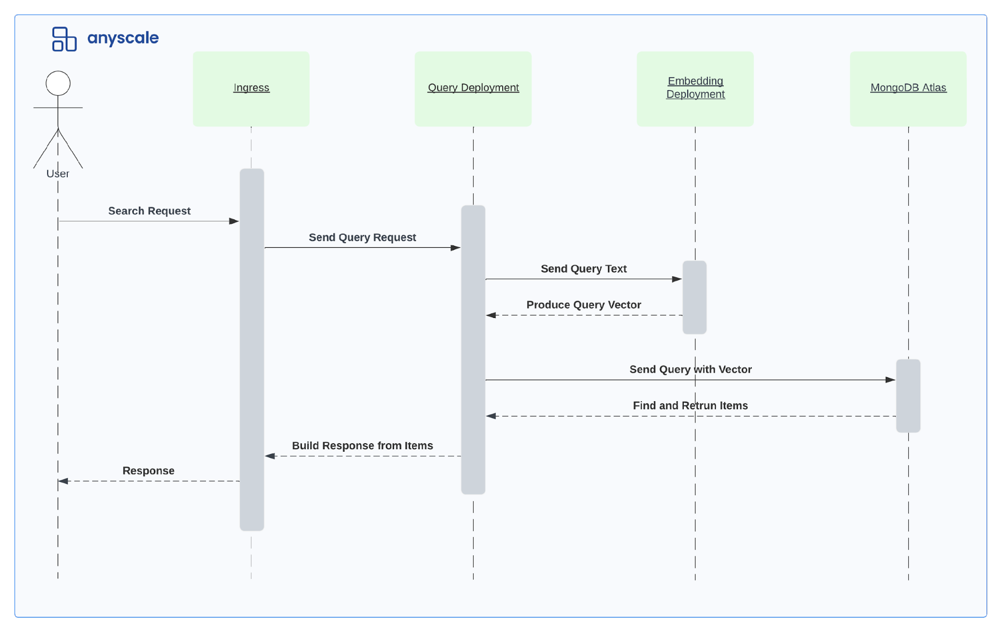
Below is a sequence diagram of the search stage showing the search request flow, which mainly involves the following steps:
Send a search request from the frontend.
Process the request at the ingress deployment.
Forward the request’s text query to the Embedding Model for generating embeddings.
Perform a vector search on the MongoDB database.
Return the search results to the ingress deployment to build a response.
Return the response to the frontend.
LinkDeep Dive: Detailed Code Walkthrough
Having gone over the high-level architecture, we will now walk through the implementation of the key components of our solution. If you want to learn how to code this yourself, read on…
LinkData Indexing: Multi-Modal Data Pipelines at Scale
We begin by detailing how to implement multi-modal data pipelines at scale. The data pipelines are designed to handle both text and image data by running multi-modal large language model instances.
LinkMetadata Enrichment: Generating Product Descriptions from Images
We make use of Ray Data to implement our data pipelines to run at scale. Ray Data is a library that provides a high-level API for building scalable data pipelines that can run using heterogeneous compute. Ray Data is built on top of Ray, a distributed computing framework that allows us to easily scale our Python code across a cluster of machines.
Below is a diagram of the data pipeline for generating product descriptions from images:
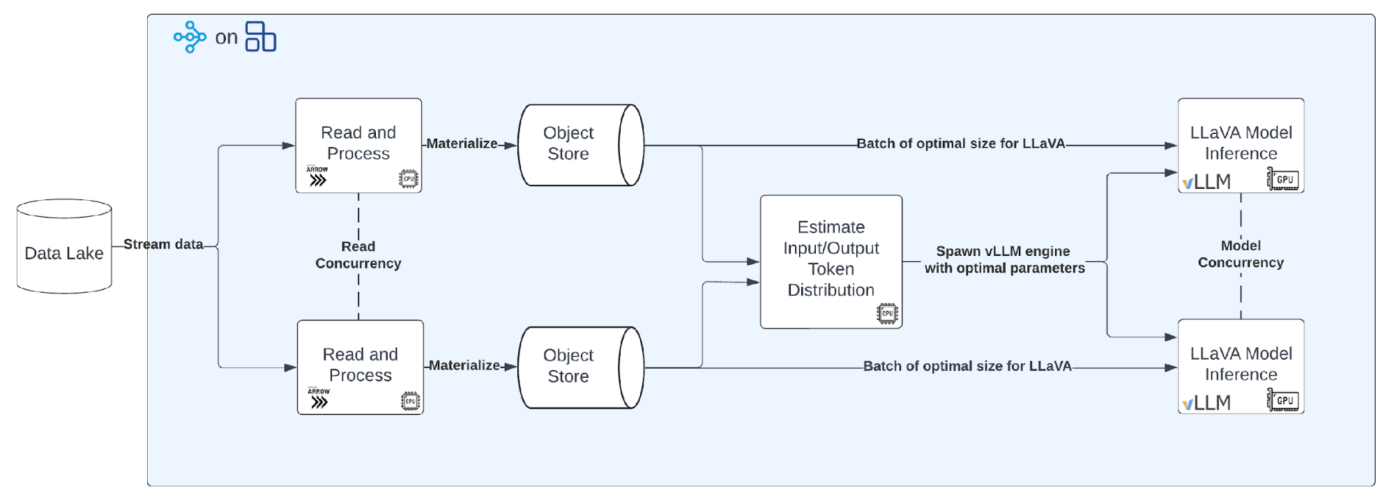
The main steps shown in the diagram are:
Read the data using pyarrow on CPUs and process it.
Estimate input/output token distribution using tokenizers on CPUs.
Run the LLaVA model inference for generating product descriptions using vLLM on GPUs.
Note that intermediate results are stored in a distributed in-memory store which is referred to as the Object Store in the above diagram.
LinkRead and Process Data
Ray Data’s API adopts lazy execution, which means that the data processing operations are only executed when the data is needed. We start by specifying how to construct a Ray Data Dataset using one of the IO connectors. We then apply transformations to the Dataset object using the map and filter operations which can be applied in parallel across the data either row-wise or in batches.
Here is the implementation of the Ray Data pipeline for reading and processing the data:
1ds = ray.data.read_csv(path, ...)
2ds = (
3  ds.map_batches(download_images, concurrency=num_download_image_workers, num_cpus=4)
4  .filter(lambda x: bool(x["img"]))
5  .map(LargestCenterSquare(size=336))
6  .map(gen_description_prompt)
7  .materialize()
8)
The above code will:
Read the data from the data lake store.
Download the images in parallel using the download_images function.
Filter out the invalid/empty images.
Crop the images to the largest center square using the LargestCenterSquare callable.
Generate the description prompt for the model using the gen_description_prompt function.
Materialize the dataset, which triggers the execution of the pipeline and storing the results in memory.
We use the llava-hf/llava-v1.6-mistral-7b-hf model for generating descriptions of products given a product image and name.
Here is the function we will use for generating prompts for the model:
1def gen_description_prompt(row: dict[str, Any]) -> dict[str, Any]:
2    title = row["name"]
3    row["description_prompt"] = "<image>" * 1176 + (
4        f"\nUSER: Generate an ecommerce product description given the image and this title: {title}."
5        "Make sure to include information about the color of the product in the description."
6        "\nASSISTANT:"
7    )
8
9    return row
map and filter take a function that operates on a single row of the dataset hence why gen_description_prompt expects a row. Whereas map_batches takes a function that operates on a batch of rows - i.e. download_images will expect a batch input instead.
For the complete implementation of the data pipeline, refer to our github repository here.
LinkEstimate Input/Output Token Distribution for LLaVA Model
We then proceed to compute input/output token distribution for the LLaVA model. This is necessary to optimally make use of vLLM, our chosen inference engine. The default input/output token distribution values assumed by vLLM leave a lot of performance on the table.
vLLM is a library for high throughput generation of LLM models by leveraging various performance optimizations, primarily:
Efficient management of attention key and value memory with PagedAttention
Fast model execution with CUDA/HIP graph
Quantization: GPTQ, AWQ, SqueezeLLM, FP8 KV Cache
Optimized CUDA kernels
Below is an animation of the generation process for a request with PagedAttention taken from the vLLM blog post. This generation process enables vLLM to optimally allocate the GPU memory when storing the KV cache for a transformer-based model, making it possible to process more sequences in parallel (i.e. unlocking memory-bound throughput bottlenecks).
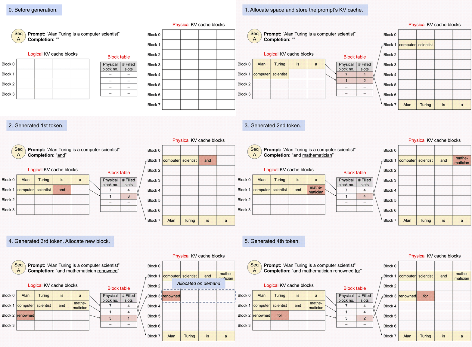
Source: vLLM: Easy, Fast, and Cheap LLM Serving with PagedAttention
Therefore to maximize the KV cache capacity, it is best to specify the maximum number of tokens that each sequence will consume. This will inform vLLM on the maximum number of blocks each sequence will consume—and thus the maximum number of sequences that can be processed in parallel.
To do so, we compute the maximum input tokens by running a LlaVAMistralTokenizer on the description_prompt field using the below code
1max_input_tokens = (
2    ds.map_batches(
3        LlaVAMistralTokenizer,
4        fn_kwargs={
5            "input": "description_prompt",
6            "output": "description_prompt_tokens",
7        },
8        concurrency=num_llava_tokenizer_workers,
9        num_cpus=1,
10    )
11    .select_columns(["description_prompt_tokens"])
12    .map(compute_num_tokens, fn_kwargs={"col": "description_prompt_tokens"})
13    .max(on="num_tokens")
14)
We set the maximum number of output tokens to 256 given we don’t want very long product descriptions. We then compute the maximum model length as the sum of the maximum input and output tokens:
1max_output_tokens = 256
2max_model_length = max_input_tokens + max_output_tokens
Now that we have computed the input/output token maximums, we can proceed to run the LLaVA model.
LinkLLaVA Model Inference
Here is the Ray Data code for running the LLaVA model:
1ds = ds.map_batches(
2    LlaVAMistral,
3    fn_constructor_kwargs={
4        "max_model_len": max_model_length,
5        "max_tokens": max_output_tokens,
6        "max_num_seqs": 400,
7    },
8    fn_kwargs={"col": "description_prompt"},
9    batch_size=llava_model_batch_size,
10    num_gpus=1,
11    concurrency=num_llava_model_workers,
12    accelerator_type=llava_model_accelerator_type,
13)
We make use of map_batches whenever we can benefit from vectorized operations on the data. This is the case with LLaVA model inference, where we can process multiple sequences in parallel on the GPU. We find a batch size of 80 to be around optimal given the GPU memory constraints of an A10 GPU and the specified engine parameters.
Where a LlaVAMistral class is defined as:
1class LlaVAMistral:
2    def __init__(self, max_model_len: int, ...):
3        self.llm = LLM(...)
4
5    def __call__(self, batch: dict[str, np.ndarray], col: str) -> dict[str, np.ndarray]:
6        prompts = batch[col]
7        images = batch["img"]
8        responses = self.llm.generate(
9            [
10                {
11                    "prompt": prompt,
12                    "multi_modal_data": ImagePixelData(image),
13                }
14                for prompt, image in zip(prompts, images)
15            ],
16            sampling_params=self.sampling_params,
17        )
18
19        batch["description"] = [resp.outputs[0].text for resp in responses]  # type: ignore
20        return batch
This is an example of a stateful transform in Ray Data, where an expensive state like loading an LLM model can be done in the constructor and then the model can be used to generate responses in the __call__ method. What this does is spawn a long-running worker process with the model loaded in memory, and then the __call__ method is called on each batch of data that is sent to the worker process.
LinkMetadata Enrichment: Generating Product Classifications from Descriptions
Here is a diagram of the data pipeline for generating product classifications from descriptions:
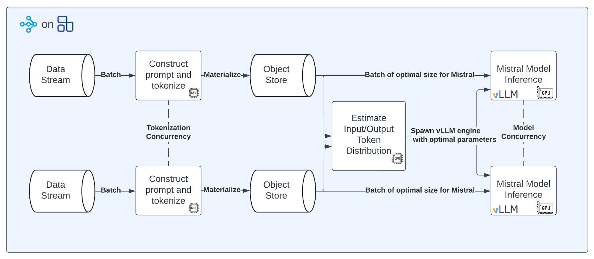
The main steps in the pipeline are:
Construct prompts and tokenize them for the Mistral model on CPUs.
Estimate input/output token distribution for the Mistral model using CPUs.
Run the Mistral model inference for generating product classifications using vLLM on GPUs
LinkConstruct Prompts and Tokenize for Mistral Model
We begin by constructing prompts for the classifiers and tokenizing them for the Mistral model. Here is the code for our classifiers specification:
1classifiers: dict[str, Any] = {
2    "category": {
3        "classes": ["Tops", "Bottoms", "Dresses", "Footwear", "Accessories"],
4        "prompt_template": (
5            "Given the title of this product: {title} and "
6            "the description: {description}, what category does it belong to? "
7            "Chose from the following categories: {classes_str}. "
8            "Return the category that best fits the product. Only return the category name and nothing else."
9        ),
10        "prompt_constructor": construct_prompt_classifier,
11    },
12    "season": {
13        "classes": ["Summer", "Winter", "Spring", "Fall"],
14        "prompt_template": ...,
15        "prompt_constructor": construct_prompt_classifier,
16    },
17    "color": {
18        ...
19    }
20}
We proceed to construct prompts and tokenize them for each classifier using Ray Data and a Mistral model tokenizer implementation
1for classifier, classifier_spec in classifiers.items():
2  ds = (
3      ds.map(
4          classifier_spec["prompt_constructor"],
5          fn_kwargs={
6              "prompt_template": classifier_spec["prompt_template"],
7              "classes": classifier_spec["classes"],
8              "col": classifier,
9          },
10      )
11      .map_batches(
12          MistralTokenizer,
13          fn_kwargs={
14              "input": f"{classifier}_prompt",
15              "output": f"{classifier}_prompt_tokens",
16          },
17          concurrency=num_mistral_tokenizer_workers_per_classifier,
18          num_cpus=1,
19      )
20      .materialize()
21 )LinkEstimating Input/Output Token Distribution for Mistral Model
Similar to the LLaVA model, we estimate the input/output token distribution for the Mistral model:
1for classifier, classifier_spec in classifiers.items():
2    ...
3    max_input_tokens = (
4        ds.select_columns([f"{classifier}_prompt_tokens"])
5        .map(compute_num_tokens, fn_kwargs={"col": f"{classifier}_prompt_tokens"})
6        .max(on="num_tokens")
7    )
8    max_output_tokens = classifier_spec["max_output_tokens"]
9    max_model_length = max_input_tokens + max_output_tokens
10 classifier_spec["max_model_length"] = max_model_lengthLinkMistral Model Inference
Lastly, we run the Mistral model inference for generating product classifications by mapping batches to the MistralvLLM stateful transform as seen in the code below:
1for classifier, classifier_spec in classifiers.items():
2    ds = (
3        ds.map_batches(
4            MistralvLLM,
5            ...,
6            batch_size=80,
7            num_gpus=num_mistral_workers_per_classifier,
8            concurrency=1,
9            accelerator_type=NVIDIA_TESLA_A10G,
10        )
11        .map(
12            MistralDeTokenizer,
13            fn_kwargs={"key": f"{classifier}_response"},
14            concurrency=num_detokenizers_per_classifier,
15            num_cpus=1,
16        )
17        .map(
18            clean_response,
19            fn_kwargs={
20                "classes": classifier_spec["classes"],
21                "response_col": f"{classifier}_response",
22            },
23        )
24    )
Note that unlike the LLaVA model, we chose to decouple the process of de-tokenization and response cleaning. We did this in order to showcase that we can independently scale processing steps within the pipeline. Ultimately, being able to decouple complex and compute intensive workloads will help unlock performance bottlenecks. This is feasible given how easily we can autoscale a heterogeneous cluster of workers with Anyscale. Anyscale will automatically scale nodes up or down with optimized start-up times to elastically right-size the cluster with GPU and CPU nodes.
To view the complete implementation of the metadata enrichment pipeline, refer to our github repository here.
LinkEmbeddings Generation and Data Ingestion
We then proceed to generate embeddings for the product names and descriptions using an embedding model.
Below is a diagram of the data pipeline for generating embeddings:
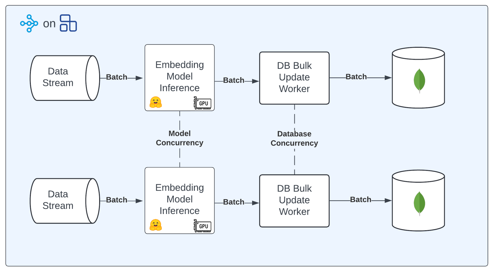
The main steps in the pipeline are:
Run the embedding model for generating embeddings.
Ingest the data into MongoDB.
LinkEmbeddings generation with Ray Data
Here is the Ray Data code for generating embeddings:
1ds = ds.map_batches(
2    EmbedderSentenceTransformer,
3    fn_kwargs={"cols": ["name", "description"]},
4    batch_size=80,
5    num_gpus=1,
6    concurrency=num_embedder_workers,
7    accelerator_type=NVIDIA_TESLA_A10G,
8)
9Where an EmbedderSentenceTransformer class is defined as:
10class EmbedderSentenceTransformer:
11    def __init__(self, model: str = "thenlper/gte-large"):
12        self.model = SentenceTransformer(model, device="cuda")
13
14    def __call__(
15        self, batch: dict[str, np.ndarray], cols: list[str]
16    ) -> dict[str, np.ndarray]:
17        for col in cols:
18            batch[f"{col}_embedding"] = self.model.encode(  # type: ignore
19                batch[col].tolist(), batch_size=len(batch[col])
20            )
21 return batchLinkData Ingestion at Scale with Ray Data and PyMongo
Finally, we proceed to ingest the processed data into MongoDB using PyMongo. Here is the Ray Data code for ingesting the data. Note that we choose to use either the MongoBulkInsert or the MongoBulkUpdate depending on whether we are performing the first run or an update to the database. We make sure to set concurrency to a reasonable value which avoids a connection storm against our MongoDB cluster. The number of connections the database can handle will depend on the size of the chosen cluster.
1mongo_bulk_op: Type[MongoBulkInsert] | Type[MongoBulkUpdate]
2if mode == "first_run":
3    mongo_bulk_op = MongoBulkInsert
4elif mode == "update":
5    mongo_bulk_op = MongoBulkUpdate
6
7(
8    ds.map_batches(update_record)
9    .map_batches(
10        mongo_bulk_op,
11        fn_constructor_kwargs={
12            "db": db_name,
13            "collection": collection_name,
14        },
15        batch_size=db_update_batch_size,
16        concurrency=num_db_workers,
17        num_cpus=0.1,
18        batch_format="pandas",
19    )
20    .materialize()
21)
Both MongoBulkUpdate and MongoBulkInsert classes make use of the PyMongo library to perform operations in bulk. Below is an example implementation of the MongoBulkUpdate class:
1class MongoBulkUpdate:
2    def __init__(self, db: str, collection: str) -> None:
3        client = MongoClient(os.environ["DB_CONNECTION_STRING"])
4        self.collection = client[db][collection]
5
6    def __call__(self, batch_df: pd.DataFrame) -> dict[str, np.ndarray]:
7        docs = batch_df.to_dict(orient="records")
8        bulk_ops = [
9            UpdateOne(filter={"_id": doc["_id"]}, update={"$set": doc}, upsert=True)
10            for doc in docs
11        ]
12        self.collection.bulk_write(bulk_ops)
13        return {}
To view the complete implementation of the data indexing pipeline, refer to our github repository here.
LinkPipeline Execution using Anyscale Jobs
We developed and tested our data pipeline on an Anyscale workspace in order to use VSCode IDE experience running against an elastic compute cluster. Now that we’ve built the pipeline, we are ready to scale it out. To do so, we use Anyscale Jobs, which is the best way to run batch workloads in production.
We can easily submit an Anyscale Job from our workspace using the VSCode terminal. All we need is a YAML configuration file, where we specify the:
Name: The name of the Anyscale job that we are launching.
Entrypoint: We want to run the
cli.pyscript which executes our pipeline.Working directory: This is the directory containing the files required to execute the entrypoint.
Requirements: Additional dependencies to be installed when setting up the job’s runtime environment.
Environment Variables: Hugging Face access token and database connection strings.
Compute config: The type and number of nodes to enable for autoscaling the cluster.
We provide our job config job.yaml file below:
1name: enrich-data-and-upsert
2entrypoint: python cli.py ...
3working_dir: .
4requirements: requirements.txt
5env_vars:
6  DB_CONNECTION_STRING: <your mongodb connection string>
7  HF_TOKEN: <your huggingface token>
8compute_config:
9  cloud: "Anyscale Cloud"
10  head_node:
11    instance_type: m5.8xlarge
12  worker_nodes:
13  - instance_type: m5.8xlarge
14    min_nodes: 0
15    max_nodes: 10
16  - instance_type: g5.xlarge
17    min_nodes: 0
18    max_nodes: 40
To submit the job in the terminal, use the following command:
1anyscale job submit -f job.yamlThis approach allows us to execute our pipeline to a managed cluster that solely contains the metrics and logs for our job. Additionally, because we’re running this job on Anyscale, Anyscale will automatically notify us of any failures and automatically retry if a failure happens.
View the below screenshot to view our job

LinkDelta Refresh at Scale
Whenever new data is made available or changes to the existing data are made, we will want to execute an Anyscale Job which will first generate new product descriptions, metadata, and embeddings and then perform bulk updates to our MongoDB collection. This is achieved by executing the same anyscale job submit -f job.yaml command but with an updated job.yaml file where the entrypoint arguments point to the new data and explicitly specify running in “update" mode.
One thing to note is that in a production setting this is usually achieved by integrating an orchestration tool of choice with Anyscale either through native integrations or programmatically using the Anyscale SDK.
LinkBuilding and Deploying the Hybrid Search Application
The search application is composed of multiple components that work together to provide a hybrid search experience. Each component is an autoscaling Ray Serve deployment that can be scaled independently to meet the demands of the system.
Below is a diagram of the search application’s backend which the user will interact with through the frontend:
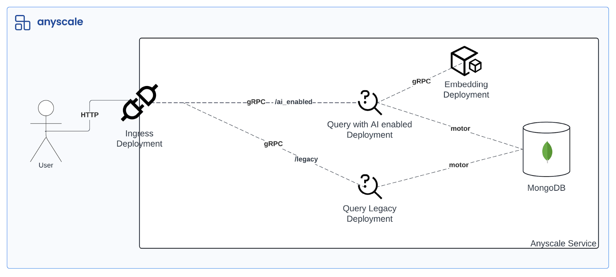
At a high level, the search backend consists of:
Ingress Deployment: Receives search requests from the frontend and forwards them to the appropriate backend deployment.
“Query Legacy” Deployment: Handles performing legacy lexical text search on the MongoDB database using motor, the asynchronous python driver for MongoDb.
“Query with AI Enabled” Deployment: Handles performing hybrid search on the MongoDB database using motor as well.
Embedding Model Deployment: Generates embeddings for the search query.
This is a sample implementation of the search backend showcasing how to compose legacy and new search capabilities through a business logic layer. By implementing custom business logic at ingress deployment, you’re able to control which users are exposed to which search capabilities. For instance, consider only wanting to expose the AI enabled search capabilities to a subset of users or only for certain queries.
LinkDefining the Ingress Deployment
Ray Serve integrates with FastAPI to provide a simple and scalable way to build APIs. Below is how we defined our ingress deployment. Note that we decorate the class with the @deployment decorator to indicate that it is a Ray Serve deployment. We also decorate the class with the @ingress decorator to indicate that it is the ingress deployment.
1fastapi = FastAPI()
2
3@deployment
4@ingress(fastapi)
5class QueryApplication:
6
7    def __init__(
8        self,
9        query_legacy: QueryLegacySearch,
10        query_ai_enabled: QueryAIEnabledSearch,
11    ):
12        self.query_legacy = query_legacy
13        self.query_ai_enabled = query_ai_enabled
14
15    @fastapi.get("/legacy")
16    async def query_legacy_search(
17        self,
18        text_search: str,
19        min_price: int,
20        max_price: int,
21        min_rating: float,
22        num_results: int,
23    ):
24        return await self.query_legacy.run.remote(...)
25
26    @fastapi.get("/ai_enabled")
27    async def query_ai_enabled_search(
28        self,
29        text_search: str,
30        min_price: int,
31        max_price: int,
32        min_rating: float,
33        categories: list[str],
34        colors: list[str],
35        seasons: list[str],
36        num_results: int,
37        embedding_column: str,
38        search_type: list[str],
39    ):
40        logger = logging.getLogger("ray.serve")
41        logger.setLevel(logging.DEBUG)
42        logger.debug(f"Running query_ai_enabled_search with {locals()=}")
43        return await self.query_ai_enabled.run.remote(...)
We define two endpoints for the ingress deployment: one for performing legacy search (/legacy) and one for performing AI-enabled search (/ai_enabled). The endpoints are defined as async functions that take the necessary parameters for the search query and return the results of the search.
To view the complete implementation of the ingress deployment, refer to our github repository here.
Link“Query with AI Enabled” Deployment
The “Query with AI Enabled” Deployment is responsible for performing hybrid search on the full MongoDB database. The search type is parameterizable as either lexical search, vector search, or both (hybrid search).
Here is how the above is controlled at the frontend:
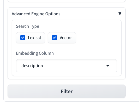
Additionally a choice of either using the generated product description or product name as the embedding field is offered.
Let’s take a look at how we can implement the Query with AI Enabled Deployment using Ray Serve:
1@deployment
2class QueryAIEnabledSearch:
3    def __init__(
4        self,
5        embedding_model: DeploymentHandle,
6        database_name: str,
7        collection_name: str,
8    ) -> None:
9        self.client = AsyncIOMotorClient(os.environ["DB_CONNECTION_STRING"])
10        self.embedding_model = embedding_model
11        self.database_name = database_name
12        self.collection_name = collection_name
13
14    async def run(
15        self,
16        text_search: str,
17        min_price: int,
18        max_price: int,
19        min_rating: float,
20        categories: list[str],
21        colors: list[str],
22        seasons: list[str],
23        n: int,
24        search_type: set[str],
25        vector_search_index_name: str = "vector_search_index",
26        vector_search_path: str = "description_embedding",
27        text_search_index_name: str = "lexical_text_search_index",
28        vector_penalty: int = 1,
29        full_text_penalty: int = 10,
30    ):
31        db = self.client[self.database_name]
32        collection = db[self.collection_name]
33
34        pipeline = []
35        if text_search.strip():
36            if "vector" in search_type:
37                embedding = await self.embedding_model.compute_embedding.remote(
38                    text_search
39                )
40
41            is_hybrid = search_type == {"vector", "lexical"}
42            if is_hybrid:
43                pipeline.extend(hybrid_search(...))
44            elif search_type == {"vector"}:
45                pipeline.extend(vector_search(...))
46            elif search_type == {"lexical"}:
47                pipeline.extend(lexical_search(...))
48                pipeline.extend(match_on_metadata(...))
49        else:
50            pipeline = match_on_metadata(...)
51
52        records = collection.aggregate(pipeline)
53        records = [record async for record in records]
54        results = [
55            (record["img"], record["name"]) for record in records
56        ]
57        return results
In the above code, here is how we implement vector search:
1def vector_search(
2    vector_search_index_name: str,
3    vector_search_path: str,
4    embedding: list[float],
5    n: int,
6    min_price: int,
7    max_price: int,
8    min_rating: float,
9    categories: list[str],
10    colors: list[str],
11    seasons: list[str],
12    cosine_score_threshold: float = 0.92,
13) -> list[dict]:
14    return [
15        {
16            "$vectorSearch": {
17                "index": vector_search_index_name,
18                "path": vector_search_path,
19                "queryVector": embedding.tolist(),
20                "numCandidates": 100,
21                "limit": n,
22                "filter": {
23                    "price": {"$gte": min_price, "$lte": max_price},
24                    "rating": {"$gte": min_rating},
25                    "category": {"$in": categories},
26                    "color": {"$in": colors},
27                    "season": {"$in": seasons},
28                },
29            }
30        },
31        {
32            "$project": {
33                "img": 1,
34                "name": 1,
35                "score": {"$meta": "vectorSearchScore"},
36            }
37        },
38        {"$match": {"score": {"$gte": cosine_score_threshold}}},
39    ]
Note we make use of the $vectorSearch aggregation stage to perform vector search on the MongoDB database. The stage takes the following parameters:
index:The name of the vector search index.path:The path to the vector field in the document.queryVector:The embedding vector of the search query.numCandidates:The number of candidates to consider for the search.limit:The number of results to return.filter:Pre-filters to apply to the search results.
Then we add a $project stage to project the fields we are interested in and a $match stage to filter the results based on the cosine similarity score.
In the above code, we also implement the lexical_search function for performing lexical search on the MongoDB database:
1def lexical_search(text_search: str) -> list[dict]:
2    return [
3        {
4            "$search": {
5                "index": "lexical_text_search_index",
6                "text": {
7                    "query": text_search,
8                    "path": "name",
9                },
10            }
11        }
12    ]
The $search aggregation stage is used to perform lexical search on the MongoDB database. The stage takes the following parameters:
index:The name of the text search index.text:The text search query and path to the text field in the document.
Note that unlike the vector search, the metadata filters are applied post the search stage when constructing a pipeline for lexical search.
In the above code, we also implement the hybrid_search function for performing hybrid search on the MongoDB database. Here is a diagram of how the hybrid search function works:
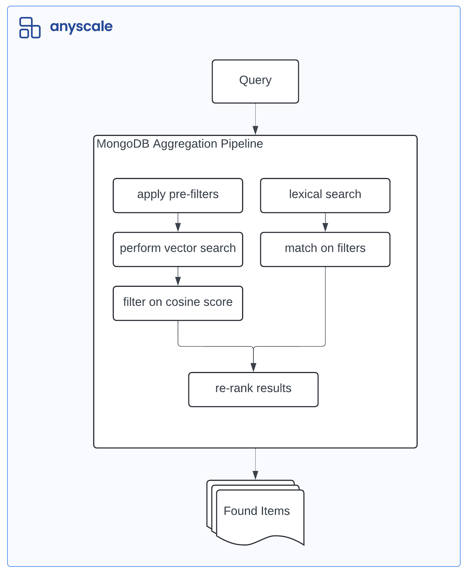
And here is how we implement hybrid search:
1def hybrid_search(
2    collection_name: str,
3    ...
4) -> list[dict]:
5    # 1. Perform vector search
6    vector_search_stages = vector_search(...)
7    convert_vector_rank_to_score_stages = convert_rank_to_score(
8        score_name="vs_score", score_penalty=vector_penalty
9    )
10
11    # 2. Perform lexical search
12    lexical_search_stages = lexical_search(text_search=text_search, text_search_index_name=text_search_index_name)
13    post_filter_stages = match_on_metadata(...)
14    convert_text_rank_to_score_stages = convert_rank_to_score(
15        score_name="fts_score", score_penalty=full_text_penalty
16    )
17
18    # 3. Rerank by combined score
19    rerank_stages = rerank_by_combined_score(
20        vs_score_name="vs_score", fts_score_name="fts_score", n=n
21    )
22
23    # 4. Put it all together
24    return [
25        *vector_search_stages,
26        *convert_vector_rank_to_score_stages,
27        {
28            "$unionWith": {
29                "coll": collection_name,
30                "pipeline": [
31                    *lexical_search_stages,
32                    *post_filter_stages,
33                    *convert_text_rank_to_score_stages,
34                ],
35            }
36        },
37        *rerank_stages,
38 ]LinkEmbedding Model Deployment
The Embedding Model Deployment is responsible for generating embeddings for the search query. Below is an example of how to define an Embedding Model Deployment using Ray Serve:
1@deployment
2class EmbeddingModel:
3    def __init__(self, model: str = "thenlper/gte-large") -> None:
4        self.model = SentenceTransformer(model)
5
6    async def compute_embedding(self, text: str) -> list[float]:
7        loop = asyncio.get_event_loop()
8        return await loop.run_in_executor(None, lambda: self.model.encode(text))
Note that depending on our traffic we can specify:
An autoscaling configuration as part of the deployment specification to scale down the embedding model to zero. This is useful in the case our expected traffic is sporadic. Scaling to zero is made easily available using Anyscale Services.
A resource type of GPU in case we want to accelerate our embedding model to process batches of incoming texts. For which we would need to dynamically batch the
compute_embeddingmethod using Ray Serve’s dynamic request batching functionality. This is useful for optimizing throughput of high volume traffic.
To view the complete implementation of the application which includes the Gradio frontend and legacy search, refer to our github repository here.
LinkSearch Application Deployment using Anyscale Services
With Anyscale Services, we can deploy highly available applications using production-ready deployment options by enabling versioned canary rollouts.
We can proceed to deploy an Anyscale Service from our workspace using the VSCode terminal. All we need is a YAML configuration file, where we specify the
Name: The name of the Anyscale service that we are deploying. If this is an existing service, then the deployment will be gradually rolled out via a canary.
Applications: The import path to both the frontend and backend applications.
Requirements: Additional dependencies to be installed when setting up the job’s runtime environment.
Flags: A flag we can set to disable authentication to our service to expose our application to the public.
We provide our service config app.yaml file below:
1name: mongo-multi-modal-search-v2
2applications:
3  - name: frontend
4    route_prefix: /
5    import_path: frontend:app
6  - name: backend
7    route_prefix: /backend
8    import_path: backend:app
9query_auth_token_enabled: false
10requirements: requirements.txt
To deploy the service in the terminal, use the following command:
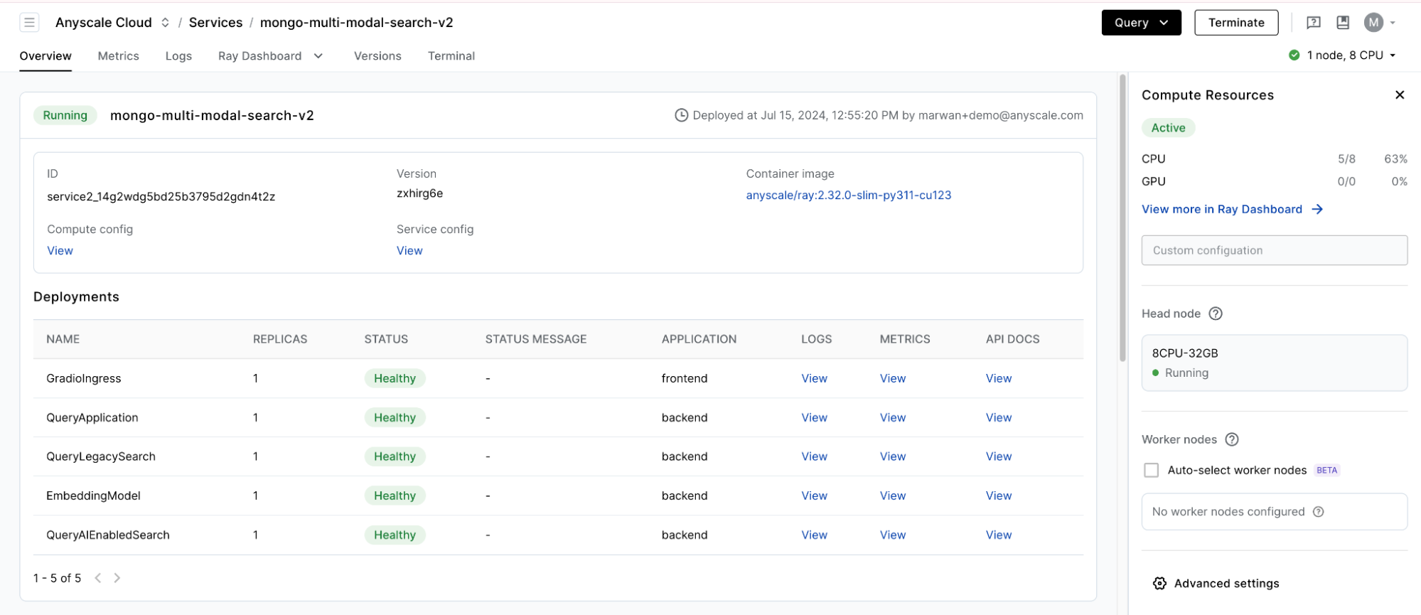
1anyscale service deploy -f app.yamlThis approach allows us to deploy our service to a managed cluster within Anyscale. Deployed service jobs have access to key performance metrics like latency, throughput, and error measures, as well as service logs.
View the below screenshot to view our deployed service:
LinkLearn More
In this guide, we have showcased a reference solution to improve a search system for multi-modal data using Anyscale and MongoDB. Additionally:
If your team is investing heavily in developing search applications, reach out to us to learn more about how Anyscale and MongoDB can help you scale and productionize your multi-modal search.
To quickly get started deploying a similar application, follow the step-by-step guide on our github repository here.
Learn more about how companies like OpenAI, Netflix, Pinterest, Verizon, Instacart and others leverage Ray and Anyscale for their AI workloads at the Ray Summit from September 30th to October 2nd.


