Many Models Batch Training at Scale with Ray Core

Batch processing is often employed when grappling with large amounts of data. Historically, this scheme has been pervasive in data engineering tasks: building scalable data pipelines; extracting, transforming, loading (ETL) data from myriad data sources into a central or common data store.

More recently, batch processing has become equally pervasive and increasingly common for machine learning training, tuning or model scoring. Simple common use cases include time-series forecasting; training hundreds or thousands of models, each model for a unique product SKU or a geographical zone, such as zip code or a pick up location, each trained on its specific batch of data; or even a unique customer id for personalized model product recommendations, each batch holding data pertinent to the unique customer id.

LinkTwo Approaches to Many-Model Batch Training

In a previous blog, we explained why train hundreds of thousands of models, why Ray is being used for these many models, and how to use different approaches with Ray Core APIs to accomplish this endeavor at scale.

source: https://github.com/justin-hj-kim/NYCtaxi_data_science

In this blog, we continue to demonstrate yet another example of how to conduct batch training on the NYC Taxi Dataset using only Ray Core and stateless Ray tasks. Because Ray tasks are asynchronous and can be embarrassingly parallelized, we will examine two approaches to employ Ray tasks to scale:

1. Distributed data loading

2. Centralized data loading

The first approach is distributed data loading. That is, delegate each independent task to read its respective batch into memory, ensuring that the desired data fits into memory. The second approach is centralized data loading. We preload each data partition once into the Ray object store, and extract each batch per location_id, store it into the Ray object store, from which each task fetches its batch data via object references, albeit at a higher cost of memory to reduce reading and training times. 

But first, let's peek at our data, understand what relationship we seek to establish among features, what transformation or projection we will need, and what features we want to train on.

LinkGlimpse at the NYC taxi data

The NYC data set contains many columns that are not of much interest to us for our task at hand, so we can discard or filter out, and only focus on columns of interest. For our use case, we want to establish a relationship between the pickup location and drop off location, and the trip duration. Because each drop off and pickup location relationship will vary at different times of the day, we need to train a separate model, each for a combination of pickup location-month combination as a batch, as shown in the Figure 1.

It turns out that the data is already partitioned into each month and year, so we can use the pickup_location_id column in the dataset to project and group it into respective data batches. Using these features, we can fit three distinct scikit-learn linear models for each batch and choose the best MAE score.

DataFrame with relevant features per pickup location id for training

LinkAnyscale Ray cluster configurations, dataset sizes, and models

We used Anyscale Ray clusters with the configurations described below for this machine learning workload. Anyscale provides a seamlessly easy way to configure, provision, launch, autoscale, and manage Ray clusters, along with insightful Ray Dashboard metrics to gauge and observe your jobs’ progress. For example, see all the Ray dashboard figures below.

Data: In all, we use 18 months of data (the year 2018 and six months of the year 2019), collectively giving us 18 files, each file with  ~7M rows, so a total of 126M rows.

Anyscale Ray cluster configuration: 

• 64 CPU cores

• 4-5 m5.2xlarge AWS EC2 instances

• 124 GiB RAM + 51.38 GiB Node memory

Models:

• Three scikit-learn model linear estimators trained and fitted for each unique pickup_locations_id

  • LinearRegression, DecisionTreeRegressor, DecisionTreeRegressor, with random splitter

• Total models trained 14100 for a total of 4700 unique pickup_locations_id

LinkApproach 1 (Distributed): A task per batch loading data into memory

In this approach, we divide our training of models into three modular and functional work:

1. Reading the parquet data

2. Creating Ray tasks to preprocess, train, and evaluate data batches

3. Dividing data into batches to spawn a Ray task for each batch 

Each of these units of functional work is modularized as a Python function, defined in mmd_utils.py.

Link1. Reading the parquet data

Using the PyArrow and Parquet push-down predicate, each task reads a parquet file, projects and extracts the batch we want to train and fit the model on, providing all the rows associated with a pickup_location_id. Achieved through the read_data() function in each Ray task, the function reads data and extracts batches separately.

1
2
3
4
5
6
7
8
9
10
11
12
13
14
15
16
17
18
19
20
21
22
23
def read_data(file: str, pickup_location_id: int) -> pd.DataFrame:
   """
   Read a file into a PyArrow table, convert to pandas and return 
   as Pandas DataFrame. Use push-down predicates since PyArrow
   supports it and only extract the needed fields, filtered
   on pickup_location_id
   Args:
       file: str path to the parquet file containing data
       pickup_location_id: int id to filter out
   Returns:
       Pandas DataFrame filtered by pickup_location_id and respective
       columns
   """
   return pq.read_table(
       file,
       filters=[("pickup_location_id", "=", pickup_location_id)],
       columns=[
           "pickup_at",
           "dropoff_at",
           "pickup_location_id",
           "dropoff_location_id",
       ],
   ).to_pandas()

By breaking into batches specific to a pickup_location_id, we avoid loading the entire partition into memory, preventing OOM errors, and extracting the desired data per pickup_location_id. Converting it to pandas allows us to train with scikit-learn estimators.

Link2. Creating Ray tasks to preprocess, train and evaluate data batches

In order to compute a trip duration, we transform our batch data pick and drop off times in standard date format to compute our duration, the time we want to predict. As part of this transformation, we fill in any missing entries. This transformation is done per task per its respective batch.

1
2
3
4
5
6
7
8
9
10
11
12
13
14
15
16
17
18
19
20
21
22
def transform_batch(df: pd.DataFrame) -> pd.DataFrame:
    """
    Given a Pandas DataFrame as an argument, tranform time format 
    for the pickup and drop times, and return the transformed Pandas
    DataFrame. Having the duration in only seconds helps for easy
    math operations.
    Args:
        df: Pandas DataFrame to be transformed
    Returns:
        a transformed Pandas DataFrame with time formats and duration
        in seconds as an additonal column
    """
    df["pickup_at"] = pd.to_datetime(
        df["pickup_at"], format="%Y-%m-%d %H:%M:%S"
    )
    df["dropoff_at"] = pd.to_datetime(
        df["dropoff_at"], format="%Y-%m-%d %H:%M:%S"
    )
    df["trip_duration"] = (df["dropoff_at"] - df["pickup_at"]).dt.seconds
    df["pickup_location_id"] = df["pickup_location_id"].fillna(-1)
    df["dropoff_location_id"] = df["dropoff_location_id"].fillna(-1)
    return df

Once transformed, we use the transformed DataFrame to fit and score the scikit-learn model and calculate the mean absolute error (MAE) on the validation set, giving us a simple regression model to predict the relationship between the pick up and drop-off location and the trip duration.

1
2
3
4
5
6
7
8
9
10
11
12
13
14
15
16
17
18
19
20
21
22
23
24
25
26
@ray.remote
def fit_and_score_sklearn(
    train: pd.DataFrame, test: pd.DataFrame, model: BaseEstimator
) -> Tuple[BaseEstimator, float]:
    """
    A Ray remote task that fits and scores a sklearn model base estimator with the train and test 
    data set supplied. Each Ray task will train on its respective batch of dataframe comprised of
    a pickup_location_id.The model will establish a linear relationship between the dropoff location
    and the trip duration.
    Args:
        train: Pandas DataFrame training data
        test: Pandas DataFrame test data
        model: sklearn BaseEstimator
    Returns: 
        a Tuple of a fitted model and its corrosponding mean absolute error (MAE)
    """
    train_X = train[["dropoff_location_id"]]
    train_y = train["trip_duration"]
    test_X = test[["dropoff_location_id"]]
    test_y = test["trip_duration"]

    # Start training.
    model = model.fit(train_X, train_y)
    pred_y = model.predict(test_X)
    error = round(mean_absolute_error(test_y, pred_y), 3)
    return model, error

Link3. Dividing data into batches to spawn a Ray task for each batch

Finally, we define a train_and_evaluate() Ray task that embodies all necessary logic to load a data batch, transform it, split it into train and test, and fit and evaluate models on it. Returning a tuple to the file path and location id used for training can map the fitted models back to pick_location_id for experimental tracking, say with MLflow or Weight & Biases.

To load and transform data, we use the read_data() and transform_batch() functions. For blog brevity, see the code details in mmd_utils.py. The driver notebook mmd_tasks.ipynb runs and trains the models in incremental batches of three files, culminating to a total of 18 files, prints the cumulative stats, and plots training times. There is an equivalent Python command line driver mmd_tasks.py that produces the same results. (See the figures below.)

Now, let's consider an optimized approach, working with the same data and workload but with lesser training times by using Ray’s object store.

LinkApproach 2 (Centralized): A task per batch loading data from Ray object store

This approach assumes two things: 1) you’ve sufficient memory for the object store and enough memory in each node in the cluster and 2) you don’t mind a higher memory cost with the merits and benefits of lower execution and training times. 

We optimize by loading and processing each partition into memory, extract all the relevant batches for the pick_location_id, and store the batches’ references into Ray’s object store.

At the heart of this optimization is the read_into_object_store() function. Four optimization techniques are used here: 1) delay calling ray.get() until necessary or when batch data is needed 2) the function yields or returns a ray.ObjectRefGenerator 3) the returned object reference generator, used as an iterator in the calling function to yield object ref, is sent to another remote Ray task train_and_evaluate_optimized.remote(...), and 4) use the SPREAD scheduling strategy to load each file on a separate node as an OOM safeguard.

1
2
3
4
5
6
7
8
9
10
11
12
13
14
15
16
17
18
19
20
21
22
23
24
25
26
27
28
29
30
31
32
33
34
35
36
37
38
39
40
41
42
43
44
@ray.remote(num_returns="dynamic")
def read_into_object_store(file: str) -> ray.ObjectRefGenerator:
    """
    This function creates a Ray Task that is a generator, returning an
    object reference generator. Read the table from the file. It stores the data
    into the Ray object store. 
    Args: 
        str path to the file name
    Returns:
        Yields Ray Object reference as tuple of pickup_id and associated batch data
    """
    # print(f"Loading {file} into arrow table")
    # Read the entire single file into memory.
    try:
        locdf = pq.read_table(
            file,
            columns=[
                "pickup_at",
                "dropoff_at",
                "pickup_location_id",
                "dropoff_location_id",
            ],
        )
        # print(f"Size of pyarrow table: {locdf.shape}")
    except Exception:
        return []

    pickup_location_ids = locdf["pickup_location_id"].unique()

    for pickup_location_id in pickup_location_ids:
        # Each id-data batch tuple will be put as a separate object into the Ray object store,
        # part of the yield statement
        # Cast PyArrow scalar to Python if needed.
        try:
            pickup_location_id = pickup_location_id.as_py()
        except Exception:
            pass

        yield (
            pickup_location_id,
            locdf.filter(
                pc.equal(locdf["pickup_location_id"], pickup_location_id)
            ).to_pandas(),
        )

Together, these optimization techniques allow for the batch data to stay in the object store until it is actually needed.

Again, for blog brevity, we refer to the relevant functions’ code defined in mmo_utils.py, particularly the read_into_object_store() and train_and_evaluate_optimized.remote(...) functions. Like its counterpart approach 1 above, there are corresponding Python drivers command line and notebook mmo_tasks.py and mmo_tasks.ipynb respectively.

With an optimized approach of using Ray’s central object store, we see an average training time per batch of files approximately 3-5X faster than the previous approach, with an incremental number of files processed. See Figure 4.

LinkObservations, Takeaways and Recap

In the Ray Dashboard screenshots for approaches 1 and 2 below, you can observe the respective difference in utilization metrics for each resource, particularly node memory and object store. 

LinkApproach 1: Distributed reads per task 

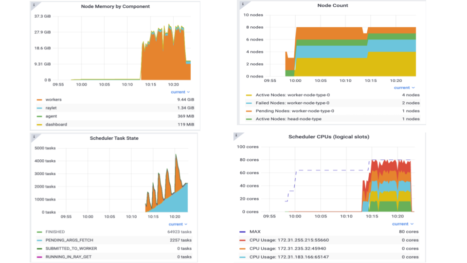Figure 1. Ray dashboard showing all the relevant metrics for approach 1.

While resources such as number of tasks, nodes, and CPU cores usage are similar across both approaches, we see more node memory consumption, hardly any Ray object store usage, and more CPU utilization, which explains why the training times take longer for approach 1.

For example, the last batch of all 18 files takes about 158 seconds to train 14100 models for a total of 4700 unique pickup locations.

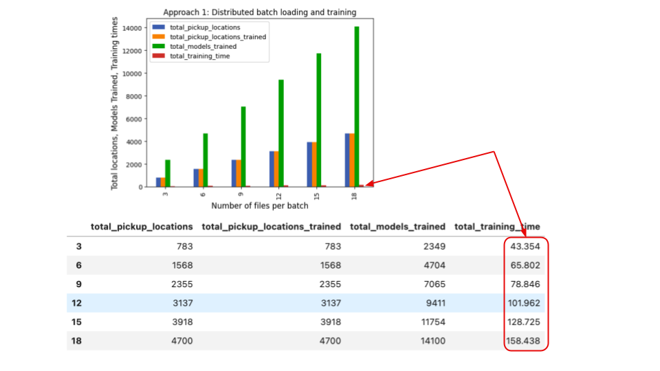Figure 2. Plots showing training times for approach 1.

LinkApproach 2: Centralized reads per task from Ray object store

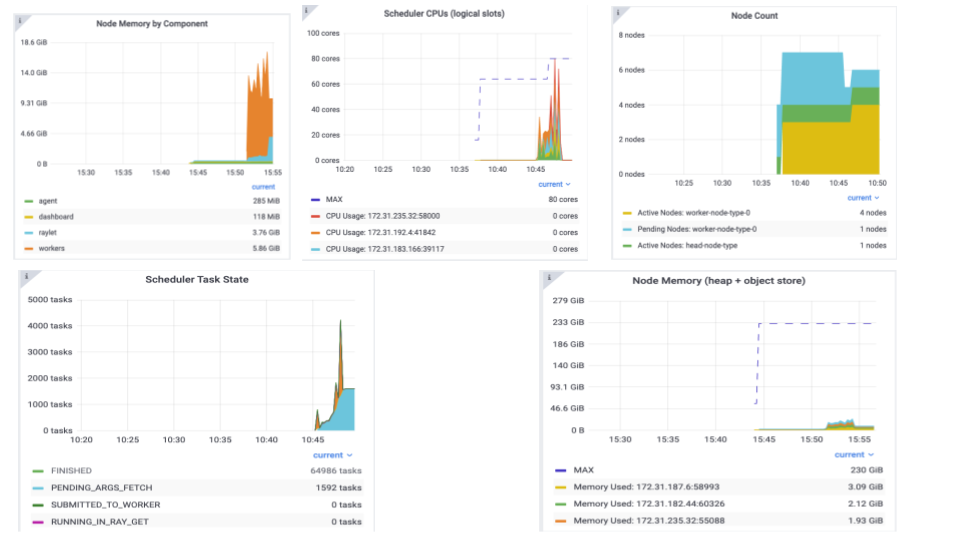Figure 3. . Ray dashboard showing all the relevant metrics for approach 2.

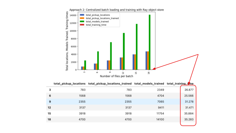Figure 4. Plots showing training times for approach 2.

By contrast, we see more Ray object store memory usage, along with node memory spikes, at a benefit of significantly lower training times, in order of ~3-5X faster. Compared to approach 1, the training time for the last batch of 18 files is only 35 seconds (hardly discernible in the above bar graph) compared to approach 1’s 158 seconds. 

Although this second approach was ~5X faster to train all models for all pickup locations, one caveat to keep in mind is that if the dataset partitions were larger and unable to fit into our cluster memory, we would have to resort to distributed reading of data, by further repartitioning parquet data files into smaller files that can fit into memory. That is, approach 1.

Both patterns, using Ray Core, are viable approaches to scale many models training on a specific feature attribute. Both patterns above showcase how to accomplish the use case and workloads to train many models to a single feature in the training set. Which one should you choose depends on your use case and size of the dataset. In either case, we recommend trying both and evaluating what works best for you, given your available cluster resources.

Lastly, if you have a similar Ray use case or story, our Ray Summit 2023 CfP is open for call to proposals. Submit your Ray story and share with the growing global Ray community. Also, we have a regular cadence of monthly Ray Meetups. Do join us to learn how the community is using Ray and Anyscale to scale their machine learning workloads.

Link
References and Resources 

• Training One Million Machine Learning Models in Record Time with Ray

• Model Batch Inference in Ray: Actors, ActorPool, and Datasets

• Batch Training with Ray Core

• Driver Notebook Approach 1 

• Driver Notebook Approach 2